1. Chapter 5 – Relations and Functions

2. 5.1Cartesian Products and Relations Definition 5.1: For sets A, B  U, the Cartesian product, or cross product, of A and B is denoted by A  B and equals {(a, b)| a  A, b  B}. We say that the elements of A  B are ordered pairs. The following properties hold: –For (a, b), (c, d)  A  B, we have (a, b) = (c, d) if and only if a = c and b = d. –If A, B are finite, it follows from the rule of product that |A  B| = |A|  |B|. We will have |A  B| = |B  A|, but not have A  B = B  A. –Although A, B  U, it is not necessary that A  B  U. –If n  Z+, n  3, and A 1, A 2, …, A n  U, then the (n-fold) product of A 1, A 2, …, A n is denoted by A 1  A 2  …  A n and equals {(a 1,a 2,…,a n )| a i  A i, 1  i  n}. –The elements of A 1  A 2  …  A n are called ordered n-tuples. –If (a 1,a 2,…,a n ), (b 1,b 2,…,b n )  A 1  A 2  …  A n, then (a 1,a 2,…,a n ) = (b 1,b 2,…,b n ) if and only if a i =b i, for all 1  i  n.

3. Example 5.1 and 5.2: page 218.

4. Definition 5.2: For sets A, B  U, any subset of A  B is called a relation from A to B. Any subset of A  A is called a binary relation on A.

5. Example 5.5: page 220.

6. Lemma: For finite sets A, B with |A| = m and |B| = n, there are 2 mn relations from A to B, including the empty relation and A  B itself. There are also 2 nm (=2 mn ) relations from B to A, one of which is also  and another of which is B  A.

7. Example 5.6: page 220

8. Example 5.7: page 220~221. (note on infix notation for a relation!)

9. Observations: For any set A  U, A  = . (If A  , let (a, b)  A  . Then a  A and b . Impossible!) Likewise,   A= .

10. Theorem 5.1: For any sets A, B, C  U: A  (B  C) = (A  B)  (A  C) A  (B  C) = (A  B)  (A  C) (A  B)  C= (A  C)  (B  C) (A  B)  C= (A  C)  (B  C)

11. 5.2Functions: Plain and One-to- One Definition 5.3: For nonempty sets A, B, a function, or mapping, f from A to B, denoted f:A  B, is a relation from A to B in which every element of A appears exactly once as the first component of an ordered pair in the relation. We often write f(a)=b when (a, b) is an ordered pair in the function f. For (a,b)  f, b is called the image of a under f, whereas a is a preimage of b. The definition suggests that f is a method for associating with each a  A the unique element f(a)=b  B. Consequently, (a,b), (a,c)  f implies b=c.

12. Example 5.9: page 223.

13. Definition 5.4: For the function f:A  B, A is called the domain of f and B the codomain of f. The subset of B consisting of those elements that appear as second components in the ordered pairs of f is called the range of f and is also denoted by f(A) because it is the set of images (of the elements of A) under f. (See Fig 5.4)This diagram suggests that a may be regarded as an input that is transformed by f into the corresponding output, f(a).)

15. Example 5.10: page 223~224.

16. Example 5.10

18. Lemma: If A = {a1,a2,…,am} and B = {b1,b2,…,bn}, then a typical function f:A  B can be described by {(a1,x1), (a2,x2), …, (am,xm)}. We can select any of the n elements of B for x1 and then do the same for x2 (so that the same element of B may be selected for both x1 and x2). We continue this selection process until one of the n elements of B is finally selected for xm. In this way, using the rule of product, there are nm = |B||A| functions from A to B.

19. Definition Definition 5.5: A function f:A  B is called one-to-one, or injective, if each element of B appears at most once as the image of an element of A. If f:A  B is one-to-one, with A, B finite, we must have |A|  |B|. For arbitrary sets A, B, f:A  B is one-to- one if and only if for all a 1,a 2  A, f(a 1 ) = f(a 2 )  a 1 =a 2.

20. Example 5.13: page 226.

21. Example 5.14: page 226.

22. Lemma: With A = {a 1,a 2,…,a m }, B = {b 1,b 2,…,b n }, and m  n, a one-to-one function f:A  B has the form {(a 1,x 1 ), (a 2,x 2 ), …, (a m,x m )}, where there are n choices for x 1 (that is, any element of B), n – 1 choices for x 2 (that is, any element of B except the one chosen for x 1 ), n – 2 choices for x 3, and so on, finishing with n – (m –1) = n – m + 1 choices for x m. By the rule of product, the number of one-to-one functions from A to B is n(n – 1)(n – 2)…(n – m + 1) = n!/(n – m)! = P(n, m) = P(|B|, |A|).

23. Definition 5.6: If f:A  B and A 1  A, then f(A 1 ) = {b  B|b=f(a), for some a  A 1 }, and f(A 1 ) is called the image of A 1 under f.

24. Example 5.15: page 227.

25. Example 5.16: page 227.

26. Theorem 5.2: Let f:A  B, with A1, A2  A. Then f(A1  A2) = f(A1)  f(A2); f(A1  A2)  f(A1)  f(A2); f(A1  A2) = f(A1)  f(A2) when f is injective. Definition 5.7: If f:A  B and A1  A, then f| A1 :A1  B is called the restriction of f to A1 if f| A1 (a) = f(a) for all a  A1. Definition 5.8: Let A1  A and f:A1  B. If g:A  B and g(a) = f(a) for all a  A1, then we call g an extension of f to A.

27. Example 5.17: page 228.

28. Example 5.18: page 228

29. 5.3Onto Functions: Stirling Numbers of the Second Kind Definition 5.9: A function f:A  B is called onto, or surjective, if f(A)=B –– that is, if for all b  B there is at least one a  A with f(a) = b.

30. Example 5.19: page 231.

31. Example 5.20

32. Example 5.21

33. Example 5.22: page 231~232.

34. Example 5.23

35. Lemma: For finite sets A, B with |A| = m and |B| = n, there are onto functions from A to B.

36. Example 5.24: page 232. (= calculate the distribution of 7 different objects into 4 distinct containers with no container left empty!)

37. Example 5.25: page 233

38. Lemma: For m  n there are ways to distribute m distinct objects into n numbered (but otherwise identical) containers with no container left empty. Removing the numbers on the containers, so that they are now identical in appearance, we find that one distribution into these n (nonempty) identical containers corresponds with n! such distributions into the numbered containers.

39. So the number of ways in which it is possible to distribute the m distinct objects into n identical containers, with no container left empty, is This will be denoted by S(m, n) and is called a Stirling number of the second kind. We note that for |A| = m  n = |B|, there are n!  S(m, n) onto functions from A to B.

40. Table 5.1

41. Theorem 5.3: Let m, n be positive integers with 1 < n  m. Then S(m+1, n) = S(m, n-1) + nS(m, n).

42. Example 5.28: page 235.

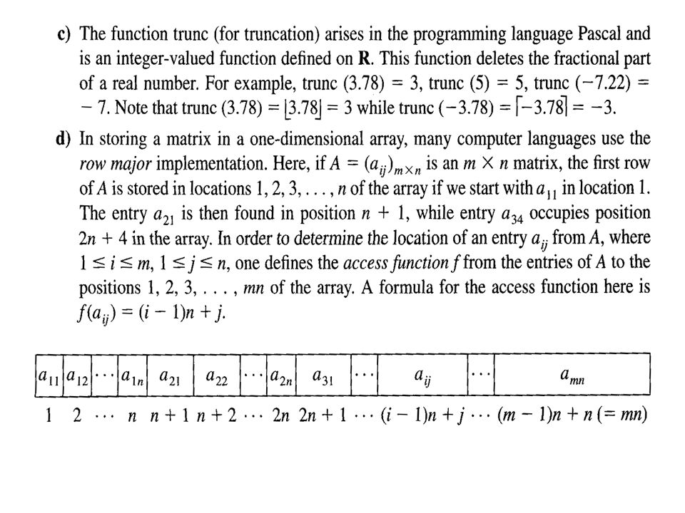
43. 5.4Special Functions Definition 5.10: For any nonempty sets A, B, any function f:A  A  B is called a binary operation on A. If B  A, then the binary operation is said to be closed (on A). (When B  A we may also say that A is closed under f.) Definition 5.11: A function g:A  A is called a uniary, or monary, operation on A.

44. Example 5.29: page 238.

45. Definition 5.12: Let f:A  A  B; that is, f is a binary operation on A. f is said to be commutative if f(a, b) = f(b, a) for all (a, b)  A  A. When B  A (that is, when f is closed), f is said to be associative if for all a, b, c  A, f(f(a, b), c) = f(a, f(b, c)).

46. Example 5.32: page 239.

47. Example 5.32: page 239

48. Definition 5.13: Let f:A  A  B be a binary operation on A. An element x  A is called an identity (or identity element) for f if f(a,x) = f(x,a) = a, for a  A.

49. Example 5.34: page 240.

50. Theorem 5.4: Let f:A  A  B be a binary operation. If f has an identity, then that identity is unique.

51. Definition 5.14: For sets A and B, if D  A  B, then  A :D  A, defined by  A (a,b) = a, is called the projection on the first coordinate. Then  B :D  B, defined by  B (a,b) = b, is called the projection on the second coordinate.

52. Example 5.36: page 241.

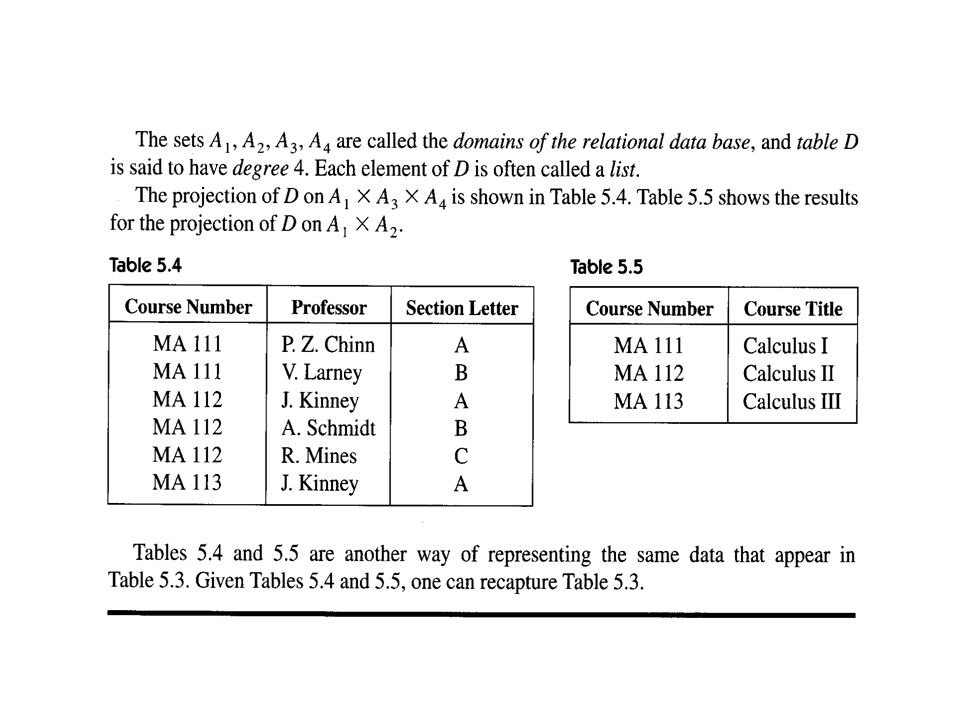
53. Lemma: Let A 1, A 2, …, A n be sets, and with and m  n. If D  A 1  A 2  …  A n =, then the function defined by is the projection of D on the i 1 th, i 2 th,…, i m th coordinates. The elements of D are called (ordered) n- tuples; an element in  (D) is an (ordered) m-tuple. (These projections arise in a natural way in the study of relational databases.)

54. Example 5.38: page 242. (applications to relational databases)

56. 5.5The Pigeonhole Principle 鴿籠原理 In mathematics one sometimes finds that an almost obvious idea, when applied in a rather subtle manner, is the key needed to solve a troublesome problem. The Pigeonhole Principle: If m pigeons occupy n pigeonholes and m > n, then at least one pigeonhole has two or more pigeons roosting in it.

58. Example 5.39: page 245.

59. Example 5.41: page 245.

60. Example 5.43: page 246

61. Example 5.45: page 246.

62. Example 5.47: page 247.

63. Example 5.48: page 248

64. 5.6Function Composition and Inverse Functions In this section we study a method for combining two functions into a single function. Then we develop the concept of the inverse (of a function) for functions. Definition 5.15: If f:A  B, then f is said to be bijective, or to be a one-to-one correspondence, if f is both one-to-one and onto.

65. Example 5.50: page 250.

66. Definition Definition 5.16: The function I A : A  A, defined by I A (a) = a for all a  A, is called the identity function for A. Definition 5.17: If f, g: A  B, we say that f and g are equal and write f = g, if f(a) = g(a) for all a  A.

67. Example 5.51: page 250.

68. Example 5.52: page 250~251.

69. Definition 5.18: If f: A  B and g: B  C, we define the composite function, which is denoted g◦f: A  C, by g◦f(a) = g(f(a)), for each a  A.

70. Example 5.53: page 251.

71. Example 5.54: page 251. For any f: A  B, we observe that f ◦ I A = f = I B ◦ f.

72. Theorem 5.5: Let f: A  B and g: B  C. If f, g are one-to-one, then g◦f is one-to-one. If f, g are onto, then g◦f is onto.

73. Example 5.55: page 252.

75. Theorem 5.6: If f: A  B, g: B  C, and h: C  D, then (h◦g)◦f = h◦(g◦f).

76. Definition 5.19: If f: A  A, we define f1 = f, and for n  Z+, fn+1=f◦(fn). Example 5.56: page 253.

77. Definition 5.20: For sets A, B  U, if  is a relation from A to B, then the converse of , denoted  c, is the relation from B to A defined by  c = {(b, a)|(a, b)   }.

78. Example 5.57: page 254.

79. Definition 5.21: If f: A  B, then f is said to be invertible if there is a function g: B  A such that g◦f = I A and f◦g = I B.

80. Example 5.58: page 254.

81. Theorem 5.7: If a function f: A  B is invertible and a function g: B  A satisfies g◦f = IA and f◦g = IB, then this function g is unique. Note: As a result of this theorem we shall call the function g the inverse of f and shall adopt the notation g = f-1. Theorem 5.7 also implies that f-1 = fc. Whenever f is an invertible function, so is the function f-1, and (f-1)-1 = f.

82. Theorem 5.8: A function f: A  B is invertible if and only if it is one-to-one and onto.

83. Example 5.59: page 255.

84. Theorem 5.9: if f: A  B, g: B  C are invertible functions, then g◦f: A  C is invertible and (g◦f) -1 = f -1 ◦g -1.

85. Example 5.60: page 255

86. Definition 5.22: if f: A  B and B 1  B, then f -1 (B1) = {x  A|f(x)  B 1 }. The set f -1 (B1) is called the preimage of B 1 under f.

87. Example 5.62: page 256

88. Example 5.63: page 257.

90. Example 2.63

92. Example 2.64

93. Theorem 5.10: If f: A  B and B1, B2  B, then f -1 (B1  B2) = f -1 (B1)  f -1 (B2); f -1 (B1  B2) = f -1 (B1)  f -1 (B2); and

94. Theorem 5.11: Let f: A  B for finite sets A and B, where |A| = |B|. Then the following statements are equivalent: (a) f is one-to-one; (b) f is onto; and (c) f is invertible.

95. 5.7 Computational Complexity For a searching algorithm, how long does it take for a success or fail search? To measure this we seek a function f(n), called the time-complexity function of the algorithm. We expect that the value of f(n) will increase as n increases.

96. Definition 5.23: Let f, g: Z+  R. We say that g dominates f (or f is dominated by g) if there exist constants m  R+ and k  Z+ such that |f(n)|  m|g(n)| for all n  Z+, where n  k. Note: When f is dominated by g we say that f is of order (at most) g and we use what is called “big–Oh” notation to designate this. We write f  O(g), where O(g) is read “order g” or “big–Oh of g”. As suggested by the notation “f  O(g)”, O(g) represents the set of all functions with domain Z+ and codomain R that are dominated by g.

97. Example 5.65: page 262.

98. Example 5.67: page 263.

99. Example 5.68: page 264.

100. Complexity Some of the most important of these orders are listed in Table 5.11.

101. 5.8 Analysis of Algorithms

102. In Fig 5.17 we have graphed a log-linear plot for the functions associated with some of the orders given in Table 5.11.

103. The data in Table 5.12 provide estimates of the running times of algorithms for certain orders of complexity.