Download presentation
Presentation is loading. Please wait.

1
Estimating Credit Exposure and Economic Capital Using Monte Carlo Simulation Ronald Lagnado Vice President, MKIRisk IPAM Conference on Financial Mathematics January 11, 2001

2
Monte Carlo Simulation for Integrated Market/Credit Risk l Random sampling generates potential future paths of market/credit risk sources l Provides time profile of credit exposure and distribution of losses l Facilitates effective management of credit limits and optimal allocation of capital

3
Benefits of Monte Carlo Simulation for Credit Risk Analysis Efficient Capital Allocation Avoid overstating credit exposure by correctly aggregating across master agreements, time, and market scenarios Account for netting, collateral, less-than-perfect correlation, mean reversion, etc. Prudent Capital Allocation Account for default correlation, risky collateral, margin call lags, correlation instability, etc.

4
MKI Integrated Risk Management Solution Consolidation Database - RV Data A P I 's ! Irregularity notifications Reports Enquirie s Limit Management RV Limits Source Systems Source Systems Source systems Source systems Manual Entry Price Feed Sources Manage Data consistent, complete, timely, accurate Collect Data Trades/deals Static Data Prices, Curves,... Distribute Information Evaluate & Monitor Risk Portfolio Analytics RV CARMA Optional Middleware

5
Time (Nodes) 1 2 3 4 5 6 7 8 9 Time Nodes Base Mark- to- Market Monte Carlo Simulation Value Begin With Current Mark-to-Market
 Time Nodes Base Mark- to- Market Monte Carlo Simulation Value Begin With Current Mark-to-Market")
6
1 2 3 4 5 6 7 8 9 Time Nodes Base Mark- to- Market Value Advance to a Future Date Monte Carlo Simulation

7
1 2 3 4 5 6 7 8 9 Time Nodes Base Mark- to- Market Value EVOLVE RISK DRIVERS Monte Carlo Simulation

8
1 2 3 4 5 6 7 8 9 Time Nodes Base Mark- to- Market Value EVOLVE RISK DRIVERS VALUE EVERY DEAL Monte Carlo Simulation

9
1 2 3 4 5 6 7 8 9 Time Nodes Base Mark- to- Market Value EVOLVE RISK DRIVERS VALUE EVERY DEAL ASSIGN TO PORTFOLIOS Monte Carlo Simulation

10
Time (Nodes) 1 2 3 4 5 6 7 8 9 Time Nodes Base Mark- to- Market Value NEW MARKET DATA VALUE EVERY DEAL ASSIGN TO PORTFOLIOS APPLY NETTING, COLLATERAL, ETC. Monte Carlo Simulation

11
Time (Nodes) 1 2 3 4 5 6 7 8 9 Time Nodes Base Mark- to- Market Value Repeat for Successive Time Nodes Monte Carlo Simulation
 Time Nodes Base Mark- to- Market Value Repeat for Successive Time Nodes Monte Carlo Simulation")
12
Time (Nodes) 1 2 3 4 5 6 7 8 9 Time Nodes Base Mark- to- Market Runs Value Distribution of Portfolio Values, Exposures, etc. Monte Carlo Simulation

13
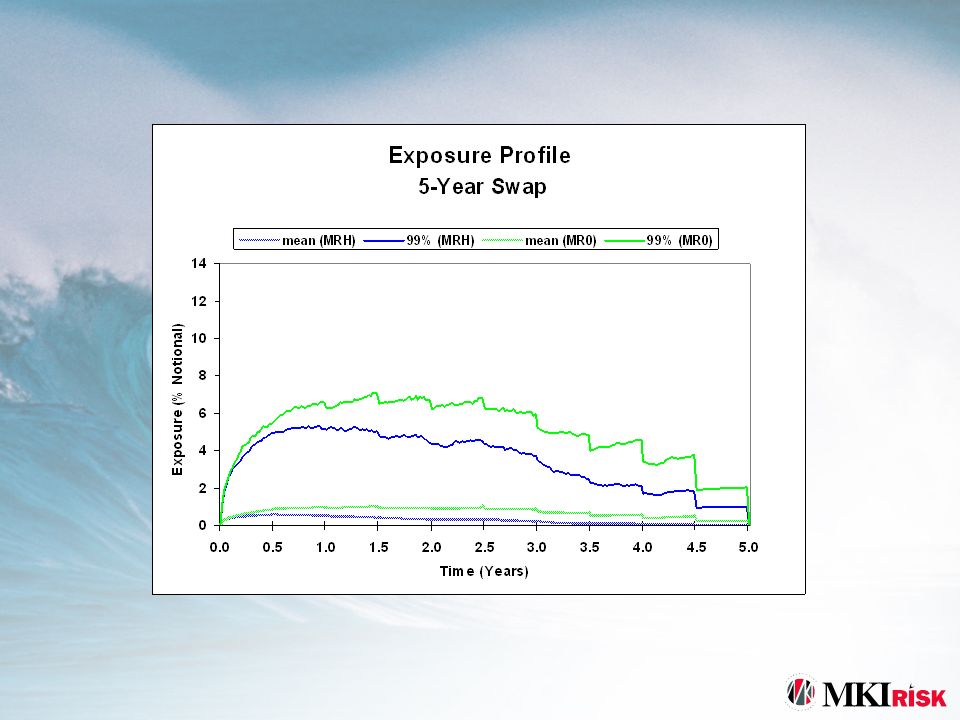
Credit Exposure Profiles Portfolio Exposure Dynamics Exposure Future Simulation Dates T 0 1 Max Exposure ‘Y’ Std Dev 1 Std Dev Mean Current Exposure Future Potential Exposure

14
Counterparty C - Guaranteed or not Master Agreement A2 Trade 10002 Trade 10001 Credit Relationships CSA A12 Counterparty B - Guaranteed or not Counterparty A - Guaranteed or not CSA A11 Trade 10003 Master Agreement A1 Collateral

15
Counterparty Exposure (Netting) Net credit exposure to Counterparty i:
 Net credit exposure to Counterparty i:")
16
Market Risk Drivers Interest Rates l Base Term Structures l Spread Term Structures Exchange Rates Equities l Indexes l Individual Stocks Commodities l Spot Prices l Forward Prices Implied Volatility Surfaces

17
Example: Interest Rate Process rvector of interest rates drivers vector of mean reversion levels Amatrix of mean reversion speeds instantaneous covariance matrix Zvector of independent Brownian motions

18
Example: Interest Rate Process Integrate over time step: discrete VAR(1) process
 process")
20
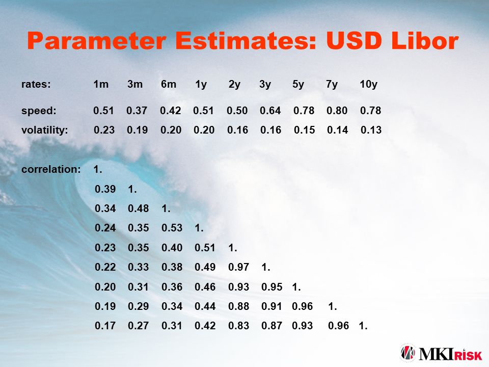
Parameter Estimates: USD Libor rates: 1m 3m 6m 1y 2y 3y 5y 7y 10y speed: 0.51 0.37 0.42 0.51 0.50 0.64 0.78 0.80 0.78 volatility: 0.23 0.19 0.20 0.20 0.16 0.16 0.15 0.14 0.13 correlation: 1. 0.39 1. 0.34 0.48 1. 0.24 0.35 0.53 1. 0.23 0.35 0.40 0.51 1. 0.22 0.33 0.38 0.49 0.97 1. 0.20 0.31 0.36 0.46 0.93 0.95 1. 0.19 0.29 0.34 0.44 0.88 0.91 0.96 1. 0.17 0.27 0.31 0.42 0.83 0.87 0.93 0.96 1.
24
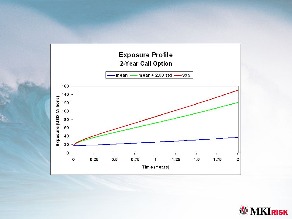
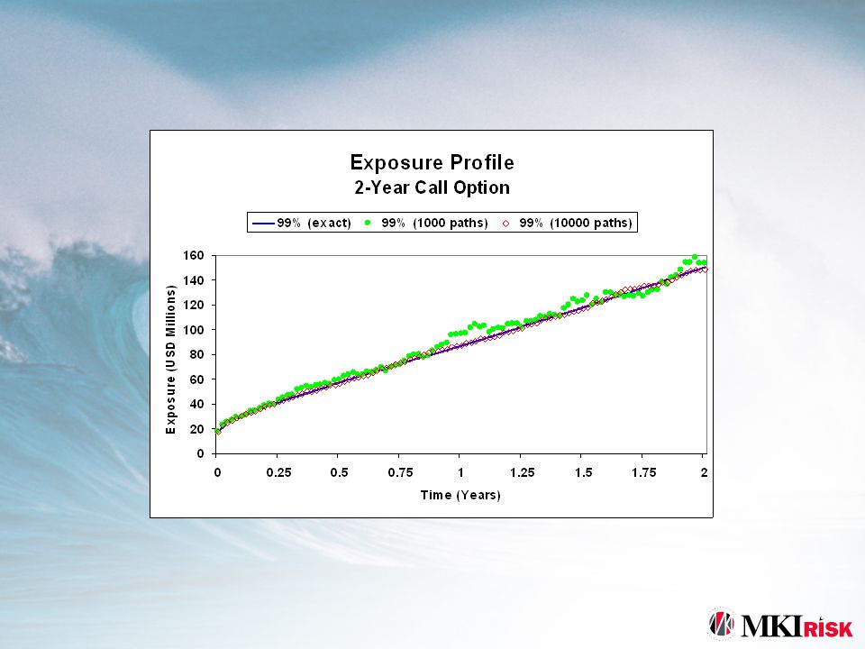
Option Exposure: Comparison of Exact Results with Monte Carlo Equity Index Call Option expiration: 2 years implied volatility: 20% initially at-the-money Underlying Stochastic Parameters drift: 15% volatility: 20% Monte Carlo Simulation: Weekly Time-Steps Exact Results: Obtained with Gauss-Hermite Quadrature

28
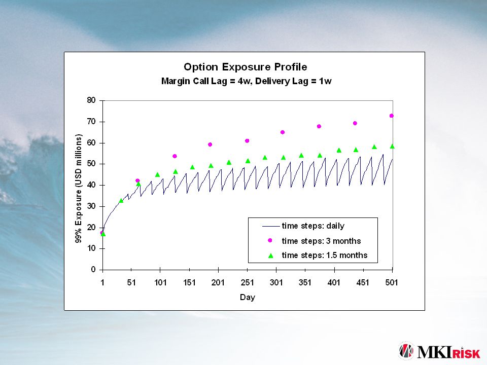
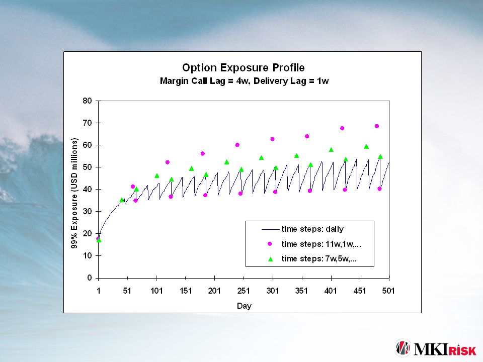
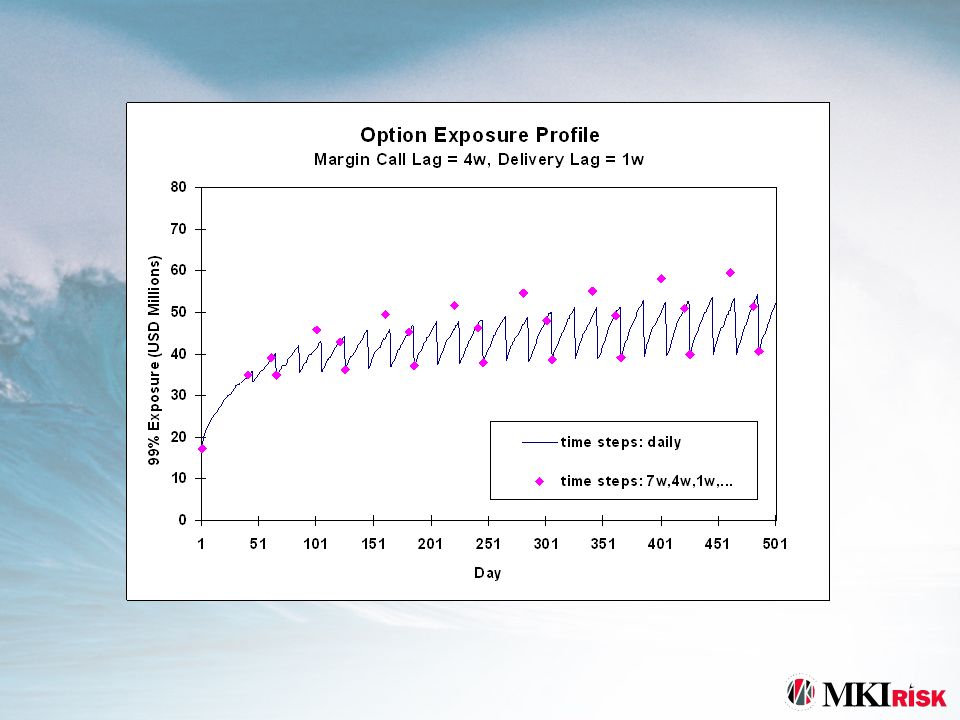
Simulation of Dynamic Collateral and Margin Call Lags Example: Single Counterparty Single Transaction: 2-year equity call option Margin Call Parameters Threshold: $30 Million Margin Call Lag: 4 weeks Delivery Lag: 1 week Excess Collateral Returned Immediately Monte Carlo Simulation: 10000 paths

32
Losses and Capital Calculation Model Requirements l l Exposure Profiles l l Credit Quality Migration and Default (Correlated) l l Stochastic Recovery Benefits l l Loss Reserves and Economic Capital l l Capital Allocation across Business Units l l Performance Measures (RAROC) l l Incremental Capital and Capital-Based Pricing
 l l Stochastic Recovery Benefits l l Loss Reserves and Economic Capital l l Capital Allocation across Business Units l l Performance Measures (RAROC) l l Incremental Capital and Capital-Based Pricing")
33
The Losses Distribution Losses PDF Distribution of Losses ( Integrated Market/Credit Risk Simulation) 0 PV(Losses))
 0 PV(Losses))")
34
The Losses Distribution Losses PDF Distribution of Losses ( Integrated Market/Credit Risk Simulation) 0 PV(Losses)) Expected Losses
 0 PV(Losses)) Expected Losses")
35
The Losses Distribution Losses PDF Distribution of Losses ( Integrated Market/Credit Risk Simulation) 0 PV(Losses)) Expected Losses Unexpected Losses
 0 PV(Losses)) Expected Losses Unexpected Losses")
36
The Losses Distribution Losses PDF Distribution of Losses ( Integrated Market/Credit Risk Simulation) 0 PV(Losses)) Expected Losses (Reserves) Unexpected Losses (Economic Capital)
 0 PV(Losses)) Expected Losses (Reserves) Unexpected Losses (Economic Capital)")
37
Credit Migration Model Markov chain with transition probability matrix: probability of migrating from rating to rating during the time interval

38
Credit Migration Model Time Inhomogeneous: Time Homogeneous:

39
Typical Transition Matrix (1-Year)
")
40
Credit Quality Migration and Default Correlation Factor Model for Asset Value Return For each counterparty

41
Credit Migration QuantilesBBB BB B CCC D A AA AAA % Change in Firm Value (Normalized) 0
 0")
42
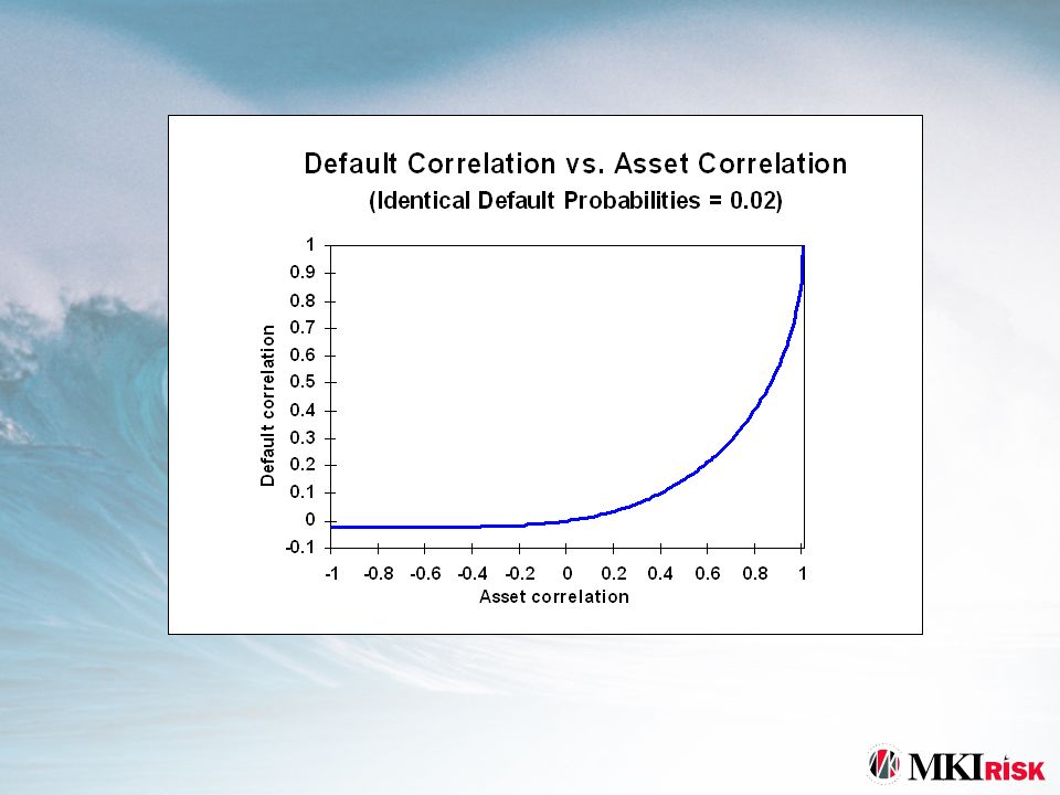
Relating Asset Returns to Default Correlation Asset-Return Correlation: Default Correlation:

44
Losses discrete time nodes: market risk driver path: idiosyncratic credit driver path: default stopping time:

45
Loss Statistics (Simplified Case) Single-period; Independent exposure and default
 Single-period; Independent exposure and default")
46
Loss Statistics (Simplified Case) Single-period Constant and identical exposures Identical default probabilities and correlations
 Single-period Constant and identical exposures Identical default probabilities and correlations")
47
Loss distributions: 500 counterparties, constant exposures, p = 0.05

48
Tolerance Intervals Ordered sample of losses from Monte Carlo simulation: Estimated quantile: Distribution of order statistics:

49
Tolerance Intervals Construct non-parametric confidence interval for estimated quantile:

50
Convergence of Unexpected Losses 500 counterparties, 550 deals, 1 year horizon

51
Summary Monte Carlo simulation is preferred approach for integrated market/credit risk analysis l Reveals distributions of future credit exposure and losses to default l Facilitates efficient capital allocation by correctly aggregating exposure across time and market scenarios l Leads to prudent capital allocation by accounting for market complexities

Similar presentations


>")
>")


 K. Cuthbertson and D. Nitzsche Lecture Credit Risk.>")
>")
