1. Daniele Montanino Università degli Studi di Lecce & Sezione INFN, Via Arnesano, 73100, Lecce, Italy daniele.montanino@le.infn.it Supernova neutrinos: oscillations and new interactions Mailny based on [ 1 ] G.L. Fogli, E.Lisi, D. M., and A. Palazzo, Supernova neutrino oscillations: A simple analytic approach, Phys. Rev. D65, 073008 (2002) (hep-ph/0111199); [ 2 ] G.L. Fogli, E. Lisi, A. Mirizzi, and D. M., Reexamining nonstandard interaction effects on supernova neutrino flavor oscillations, Phys. Rev. D66, 053010 (2002) (hep-ph/0202269); [ 3 ] G.L. Fogli, E. Lisi, A. Mirizzi, and D. M., Analysis of energy- and time-dependence of supernova shock effects on neutrino probabilities, Phys. Rev. D68, 033005 (2003) (hep-ph/0304056v2 ); [ 4 ] G.L. Fogli, E. Lisi, A. Mirizzi, and D. M., in preparation. Notice: many of the transparencies shown in this talk have been “cropped” from some Georg Raffelt’s presentations. Copy of them can be found at the following address: http://wwwth.mppmu.mpg.de/members/raffelt/

17. SN neutrino oscillations The SN ’s give us the unique possibility to probe both the “solar” and the “atmospheric”  m 2 ’s with the same “neutrino beam”. In fact: When neutrinos moves from the neutrinosphere (the start of the free streaming) to the surface of the star, the potential V(x) varies from  10 -2 eV 2 /MeV to 0, thus crossing zones with V(x)  m 2 atm /2E (“higher” transition) and V(x)  m 2 sol /2E (“lower” transition). SN neutrinos are sensitive to values of the mixing matrix element U 13 up to 10 -3, beyond of the range of the current and planned terrestrial experiments. Shock wave effects can affect the temporal structure of the signal. For these reasons, a general treatment for the calculation of the relevant e  e survival probability P ee is highly desirable.

18. Framework We have now compelling evidence that the Hamiltonian of flavor evolution: i  H    d  dt is non-trivial: H  ≠ E    Barring LSND data, all differences from triviality (  massless neutrinos) are consistent with a 3 oscillation framework: UM 2 U 2E  h(x) 3333 kinematical mass-mixing term dynamical term (in matter) + H   ( H kin + H dyn )    Mixing parameters: U = U (  12,  13,  23,  ) as for CKM matrix with  ij  without loss of generality. The parameter  23 and the CP violating phase  are irrelevant for SN neutrinos.

19. e 2 1 3  12  13 U e1, U e2, U e3 = cos  12 cos  13, sin  12 cos  13, sin  13 “Geometrical” meaning of the mixing angles Sometimes  12 is denoted with  and  13 with 

20. Mass-gap parameters: M 2  diag , ,   m 2 m2m2 2 m2m2 2 “solar” “atmospheric” Should be set by direct mass measurements: conventional zero   -decay  0 2  -decay  cosmology normal hierarchy inverted hierarchy m2/2m2/2 -m2/2-m2/2 m2m2  m 2 m2/2m2/2 -m2/2-m2/2 2 2 1 1 3 3 Dynamical term: V(x) 0 0  V(x)    where V(x)  2G F N e (x)  7.6  10 -6 eV 2 /MeV  (x)/g·cm -3 is the neutrino potential in matter (“  “ for neutrinos, “  “ for antineutrinos). h(x)     standard (MSW) term non-standard term

21. Remarks For the oscillation parameters reported above, the relevant transitions take place far from neutrinosphere, were incoherent and - scattering can take place [see e.g., S. Pastor, G. Raffelt, Phys. Rev. Lett. 89, 191101 (2002)]. Since |  m 2 |>>  m 2, (“one-mass scale dominance”) the 3 problem can be decoupled into two effective 2 problems: S 3 (  m 2,  m 2,  12,  13 )  S 2 (  m 2,  12 )  S 2 (  m 2,  13 ). The 2  2 mixing matrix can be written as: cos  sin   sin  cos  U   The only relevant probability for supernovae is the P ee  P( e  e ) : F e  P ee F e 0 + (1  P ee ) F x 0 F   F   (1  P ee ) F x 0  (1  P ee ) F e 0 (F x 0  F  0  F  0 )

22. Static neutrino potential [T. Shigeyama and K. Nomoto, Astophys.J. 360, 242 (1990)] Power-law parameterization:  1.58  10 -8 x R sun -3 V (x) eV 2 /MeV where R sun  6.96  10 5 km is the solar radius.

23. Standard approach to SN (and solar) oscillations i  H    d  dt Take the evolution equation in matter: Diagonalize the Hamiltonian: U m ·H(x) · U m  diag M 1 (x) 2, M 2 (x) 2, M 3 (x) 2 + Write the neutrino “eigenstates” in matter: m i  U m i   + Rewrite the evolution equation in this basis: i   M i 2  i j - m j d m i dt dU m dt UmUm + ij 1 2E The term U + m dU m /dt is generally much smaller than the first, except near to the points when M 1 (x L ) 2 ~ M 2 (x L ) 2 (lower resonance) and M 2 (x H ) 2 ~ M 3 (X H ) 2 (higher resonance). Far from these two points, the eigenstates in matter are conserved (adiabatic propagation). In the lower (higher) resonance points there is a non-zero probability for a m 1  m 2 ( m 2  m 3 ) transition.

24. rotation to eigenstates in matter (at the neutrinosphere) higher transitionlower transitionrotation to the original flavor basis P L =P c ( m 2  m 1 )P H =P c ( m 3  m 2 ) Mm2Mm2 V(x) -m2-m2 +m2+m2 m2m2 3 2 1 m 3 m 2 m 1 Crossing points lower crossing pointhigher crossing point Toward Earth Toward SN core V(x L )  k L =  m 2 /2EV(x H )  k H =  m 2 /2E

25. Mm2Mm2 V(x) -m2-m2 +m2+m2 m2m2 3 2 1 m 3 m 2 m 1 Mm2Mm2 V(x) 3 2 1 m 3 m 2 m 1 Normal hierarchy Mm2Mm2 V(x) -m2-m2 +m2+m2  m 2 3 2 1 m 3 m 2 m 1 Inverted hierarchy P H =P ( m 3  m 2 ) P L =P ( m 2  m 1 ) P L =P ( m 1  m 2 ) Mm2Mm2 V(x) 3 2 1 m 3 m 2 m 1 P L =P ( m 2  m 1 ) P L =P ( m 1  m 2 ) P H =P ( m 3  m 1 ) neutrinosantineutrinos

26. U 2 m,e1 U 2 m,e2  U 2 m,e3 cos 2  m 12 cos 2  m 13 sin 2  m 12 cos 2  m 13 sin 2  m 13 where k H  m 2 /2E and k L  m 2 /2E, and V NS is the potential at the neutrinosphere (i.e., at the starting of the free streaming of neutrinos) Since the neutrino potential at the neutrinosphere is much larger than the squared mass gaps: V NS >>  m 2 >  m 2, we can tend V NS to infinity: where k H >0 (k H <0) for normal (inverted) hierarchy and the minus (plus) sign holds for neutrinos (antineutrinos). Consequently we have: U 2 m,e1 U 2 m,e2  U 2 m,e3 001001 for  ’s and normal hierarchy or  ’s and inverted hierarchy; 100100 for  ’s and normal hierarchy; 010010 for ’ s and inverse hierarchy. = =

27. Calculation of the crossing probability The crossing point x c should be chosen as the point where the adiabaticity condition is maximally violated. It can be proved that this point correspond with a good approximation to the point where: V(x p )  k A widely used formula for the calculation of the crossing probability is the double-exponential: P( a m  b m )  P c (k,  )  exp(2  rkcos 2  )  1 exp(2  rk)  1 where k  m ab 2 /2E is the vacuum oscillation wavenumber and r is a scale factor, i.e., the inverse of the logarithmic derivate of the potential V(x) in the crossing point x p : r  dV(x) 1 V(x) dx x=x c 

28. Phenomenological inputs  m 2  (7.0  0.8)  10 -5 eV 2 sin 2  12   0.3  0.03 sin 2  13  0.022  m 2  (2.0  0.4)  10 -3 eV 2 (at 1  ) From solar and atmospheric (+K2K +KamLand +CHOOZ) analysis: we have that P L ( )  P L ( )  0 and: P H  exp(  2π r H k H sin 2  13 )  Collecting all the previous recipes, we have that the analytical form of P ee becomes exceedingly simple: P ee (E)  sin 2  12 P H (E) (, normal hierarchy) cos 2  12 (, normal hierarchy ) sin 2  12 (, inverted hierarchy ) cos 2  12 P H (E) (, inverted hierarchy )  Landau Zener approximation

29. The Earth effect If the detector is the Earth shadow with respect to the supernova, the neutrinos cross the Earth before reach the detector. Under the assumption  m 2 <<  m 2, we have simply to replace sin 2  12  P E  P (2 ) ( e  2 ). The quantity P E can easily calculated analytically assuming two shells (Core and Mantle) with constant density in the Earth.

30. 3 survival probability Black (solid) line: P 3 ee survival probability, no Earth effect Red (dotted) line: P 3 ee survival probability, with Earth effect (8500km, mantel)  In principle, both hierarchy and the mixing angle  13 can be probed by SN neutrinos.  =  13  =  12  =  13  =  12 Solar+KamLand solutions

31. Effect of non-standard interactions The net effect in ordinary matter is to provide to the standard potential matrix h(x)  diag ( V(x), 0, 0 ) an extra potential of the kind: Several extension of the Standard Electroweak model (e.g., R SUSY) allow new four-fermions interactions with an effective flavor changing and flavor diagonal interaction Hamiltonian. (f = e, u, d)   ff G f 

32. We make the following simplifying assumptions: 1)   are taken real:     2) possible variations of the N e /N p ratio are neglected, so that the ∂   /∂x  0 3) |   |<<1 (say, |   |< few  10 -2 ), in agreement with the phenomenology Within the previous hypotheses, the potential matrix h+  h can be diagonalized through a matrix U(   ). In this way the MSW equation in matter can be formally cast in its standard form, modulo the replacement   ea. The final result is the following: i.e., the net effect is a shift of the angle  in the calculation of the crossing probability P c.

33. with 3 generations, by factorizing the dynamics in the “high” and “low” subsystems, we obtain that the net effect is a shift in the angle  13 (  12 ) in the calculation of the higher (lower) crossing probability: P H ( ) = P c (k H,  13 +  H ) and P L ( ) = P c (k L,  12 +  L ) where  H and  L are linear combinations of the  ai ’s: The net effect is thus a sort of dangerous “confusion scenario”, in which could be difficult (if not impossible) to disentangle the effects of the pure mixing from those coming by non standard interactions.

34. Black (solid) line: P 3 ee survival probability, no Earth effect Red (dotted) line: P 3 ee survival probability, with Earth effect (8500km, mantel)  =  13  =  12  =  13  =  12  3 survival probability (with NSI)

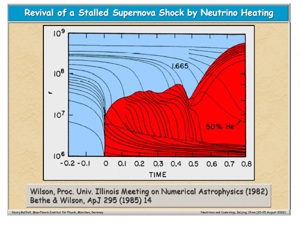
35. (*) see, e.g., R.C.Schirato, and G.M.Fuller, astro-ph/0205390 It has been realized that a prompt SN shock propagation can produce interesting effects in the energy and time structure of the signal (*). Calculation of effects is nontrivial, since the matter density profile is non monotonic and time- dependent step-like at the shock front Rarefaction zone Shock front Progenitor static profile Shock wave effect

36. Neutrino wavenumbers “Low” : k L =  m 2 /2E “High” : k H =  m 2 /2E As usual, matter effects are expected to play a significant role when V(x) ~ k H or V(x) ~ k L The latter condition has little phenomenological relevance and hereafter will be neglected. Our parameterization of the shock –wave front

37. One can have V(x)~ k H up to four times along the shock wave profile, leading to four level crossing probabilities in the “H” subsystem The crossing probabilities P i =P H (x i ) occur at points where V(x) is smooth (finite gradient) and the crossing probability can be calculated with the usual Landau Zener approximation. V(x) x1x1 x2x2 xsxs x3x3 Top of shock front Bottom of rarefaction zone P s occurs at the step-like shock front. In this extreme non adiabatic limit where  ± is the effective 1-3 mixing angle in matter just before (+) and after (-) the shock front. xbxb kHkH

38. Assuming factorization of all 4 the crossing and complete averaging over relative phases, one gets the total crossing probability P H in the H subsystem from: Q: How good is the above approximation? To check it, we have compared our analytical calculation of P H with the results of the numerical evolution of equations in the domain of energy [P H (E)] and of time [P H (t)]. The two results are in perfect agreement. P H =P H (P 1,P 2,P s,P 3 ) is a simple (polinomial) combination of the P i and P s

39. Consequences for the observables We have studied the effect of the shock propagation on the energy and time spectrum of positrons detectable through the inverse  decay: e  p  n  e + We have assumed a SN at a distance D  10 kpc, releasing a total energy E B  3  10 53 erg, equally shared among all the (anti)neutrino flavors, and exponentially decaying in time: Moreover, we have assumed for each flavor  an unpinched Fermi-Dirac spectrum with time independent temperature T  :

40. where F e (E ) is the oscillated time- dependent flux of e ’s at Earth: The positron energy spectrum is given by The size of the detector is assumed 32 kton of water (as in the Super- Kamiokande experiment. We assume, for simplicity, perfect energy resolution and zero- threshold. (normal) (inverted)

41. Time dependent spectral deformation on e with inverted hierarchy. But: Earth matter crossing might make difficult to identify shock- dependent deformation Possibility of mass hierarchy discrimination The shoulder drifts to higher energy with the passage of time

42. xbxb xsxs For e with inverted hierarchy there is a deviation w.r.t. the pure exponential drop of the luminosity Very interesting chance to extract information on  13 and on mass hierarchy. Deviation in rate are very sensitive to  13 The shock wave propagation can be followed in real time

43. Partial Conclusions Supernova neutrinos oscillations are the “next frontier” of the neutrino (Astro)Physics. In fact they can probe: the neutrino mass hierarchy as well as the mixing matrix element U 13 (or, equivalently, the mixing angle  13 ); the internal structure of the exploding supernova (e.g., prompt shock wave propagation) and shed light on the mechanism of the explosion; …but we need: larger and more sensitive detectors; better SN models A lot of patience!

44. The relic SN neutrino background Future experiments will be able to measure the background of neutrinos produced by all the past supernovae in the Universe (Supernova Relic Neutrinos, SRN)

45. The number flux of SRN of a given specie  is given by: where H(z)=H 0 [(1+  m z)(1+z) 2   z(2+z)] 1/2 is the Hubble constant as function of the redshift z (we do not consider a dynamical cosmological constant), Y  (E)=∫ dt L  (E,t) is the total yeld (total time integrated luminosity) for a typical supernova of the specie , and R SN (z) is the Supernova rate per comoving volume. R SN (z) adapted from Porciani & Madau astro-ph/0008249 (for  m =1,   =0 and H 0 =70kmMpc -1 s -1 )

46. The predicted total flux of e (the only that can be detected, due to the extremely low flux) in absence of oscillations and other effects is: where E b is the average supernova binding energy and  E e  is the initial average energy of e ’s SuperKamiokande collaboration has recently tried to measure this flux (Malek et al., hep-ex/0209028). Unfortunately, the signal is dominated by the solar neutrinos and the low energy atmospheric neutrinos, and only an upper bound can be fixed: In the future a salt of gadolinium (a neutron absorber) will be added in SK, so that the neutron produced in the inverse beta decay can be detected. In this way, most of the signal can be disentangled by the background. Moreover, bigger detectors (UNO, HyperKamiokande) are planned. GOOD CHANCE TO OBSERVE THE SRN

47. What we can learn from the SRN: we can obtain information on: Star formation rate Cosmological parameters Neutrino masses and mixing Neutrino temperatures but also on long distance neutrino properties, in particular neutrino decay The most stringent limit on decay comes from the SN1987A: where  is the rest frame neutrino lifetime. The SRN offer the possibility to prove a decay time of the order of ~1/H 0 ~10 17 s, i.e. In the following we fix H 0 =70kmMpc -1 s -1,  m =0.3 and   =0.7.

48. The initial condition: we stick in the current phenomenology of masses and mixings. We assume the Raffelt-Janka parameterization for the initial flavor spectrum: with  E e  =12MeV,  E e  =15MeV and  E x  =18MeV and  =4. Using the values of mixing angles at the neutrinosphere: and the approximation P L =0 we have for the i yelds at the surface of the supernova: ’s normal hierarchy inverted hierarchy In the following we consider, for simplicity, only the two limiting cases P H =0 or P H =1.

49. The no decay case: in this case, since sin 2  13 is very small, the e flux is given by: (Earth and shock wave effects on SRN are completely negligible, as we proved). In the case of no-decay, the result is independent from the cosmological parameters. Notice that the case of Normal Hierarchy (NH) and Inverse Hierarchy (IH) with P H =1 are indistinguishable.

50. SRN decay: general formalism: The equation governing the number density n i (per comoving volume) of the mass eigenstate i is the Boltzmann equation: where  i =1/  i is the decay amplitude of the state i [  i =0 for the lightest state(s)], and q ij is the contribution to n i due to the decay of the heavier j states [q ij =0 for the heaviest state(s)]: where b i  j and  i  j are respectively the branching ratio and the normalized spectrum of the decay i  j. These equations can be easily solved with the substitution z=z(t) and  =E/(1+z).

51. The solutions of the Boltzmann equation is with: These integral can be calculated in sequence from the heaviest state(s) to the lightest state(s). Of course, the e flux on the Earth (neglecting Earth matter effects) is given by: The previous equations reduce to no decay case in the limit  i  0. Notice that we do not consider possible interference effects between oscillations and decay. This is a very good approximation in the actual phenomenology (see Lindner et. al. astro-ph/0105309).

52. The majoron decay: among all the possible neutrino decay scenarios, we consider a decay in an invisible massless (pseudo)scalar particle, usually called “majoron”: j  i +  mediated by a renormalizable interaction lagrangian: ( ) where the i states are majorana states. For simplicity we consider only the two limiting cases: b j  i  j  i (E i,E j ) 1) m j >> m i “1/2” 2E i /E j 2 2/E j (1  E i /E j ) 2) m j >m i “1”0  (E j  E i ) - ~

53. Normal Hierarchy (NH) Inverted Hierarchy (IH) 3 decay scheme: within the phenomenology, we have 3 limiting cases: 1 2 3 1 2 3 2) m 3 >> m 2 >> m 1 1/4 1/2 1 2 3 1 2 3 1) m 3 >m 2 >m 1 ~~ 1/2 11 Branching ratios We assume absence of CP violations in the decay and that all the decay channels for each state i are equally shared. Moreover, we assume an equal  /m for all the decaying states. In the IH scenario, due to the smallness of  13 the cases m 1,2 >> m 3 and m 1,2 >m 3 are essentially indistinguishable. 3 2 1 3 2 1 1/2 (1/3) 1/2 (1/3) 1/2 (1/3) 1 (1/2) 1 (1/2) ~ m2m2 m2m2  1 /m 1 =  2 /m 2  /m  3 /m 3 =  2 /m 2  /m 0

54. Complete (“fast”) decay case: if  E/m >> 1/H 0 we expect that almost all the states have decayed into the lightest state(s) before reach. In this limit, the result is independent from the value of  /m. In particular, in the IH scenario all the states have decayed into the (invisible) 3 : in this case we expect the complete disappearance of the signal. In the NH scenario, we have: where Y eff e is the “effective” yield of e produced by a Supernova. We have to distinguish the two subcases: ~~ 1) m 3 >m 2 >m 1 (nearly degenerate case): in this case the 1 daughter neutrinos preserve the energy of the parent one, and there are no cross decays:

55. 2) m 3 >> m 2 >> m 1 : in this case we have: where the operators D and D are defined as: With the Raffelt-Janka parameterization and in the limit P H =0 or P H =1 these integrals can be calculated analytically. As we can see, the cases P H =0 or P H =1 are almost indistinguishable.

56. Results: we have seen that in the case of complete decay we can have either a complete disappearance of the signal (in the case of Inverse Hierarchy) or an enhancement of the signal by a factor 2 (in the case of quasidegenerate Normal Hierarchy). The case of incomplete decay should interpolate between the complete decay and no decay cases. We choose  /m=7  10 10 s/eV as intermediate decay time. NH, quasidegenerate

57. NH, m 3 >> m 2 >> m 1 IH The enhancement at low energy is suppressed by the ~E 2 dependence of the cross section

58. Since in the near future, only the absolute flux will be measured, we consider the total number events (normalized to the no oscillations case) in the positron energy window [10,20]MeV as function of  /m The NH case with m 2 >> m 2 >> m 1 (green line) is almost indistinguishable from the no oscillation case for all values of  /m. The quasidegenerate NH case (red line) or the IH cases (blue and dashed lines) can be be proved, by an enhancement or a diminution of the signal, respectively.

59. Conclusions Supernova Relic Neutrino background is a guaranteed signal that has good chances to be discovered (and measured) in the next few years. However this signal is affected by uncertainties on cosmological and supernova parameters, as well as on the mass and mixing parameters. However, SNR can be used to study long distance neutrino properties, in particular decay. We have seen that, in some situations, a signal of decay can be well identified as an enhancement or diminution (respect to the no- decay case) of the number of SRN events in the detector. In absence of decay evidence, a limit on the decay time ~ 5 order of magnitude greater than present limit can be fixed, but only if the true neutrino mass hierarchy is known.