Download presentation
Presentation is loading. Please wait.

1
6.3 Separation of Variables and the Logistic Equation

2
Separation of variables is the what we refer to as the process of solving for an equation that satisfies a differential equation. If you remember back to section 6.1 we were asked if some function was a solution of some D.E. What we would do is take the derivative of the function and replace both the function y and y’ back into the D.E. and see if it was a solution. This process will give us the ability to determine y, so that the authors do not have to provide it for us.

3
Ultimately what we will be doing is getting all the x’s on one side with all the dx’s. The other side will contain all y’s and dy’s. You must re- write every y’ as dy/dx. Then we will integrate both sides and hopefully come up with a solution to D.E.

4
Add x to both sides Divide both sides by y Re-write right hand side using exponent rules Multiply both sides by dx Divide both sides by y -1. Re-write left hand side Show that NOW BOTH VARIABLES HAVE BEEN SEPARATED, WE CAN NOW INTEGRATE BOTH SIDES WITH RESPECT TO Y AND X.

5
Both sides could be written with +C but remember C is a constant and if we took C from the left and subtracted from the C on the right we would end up with a new C. So just to save time always put C with the x integral Now simply solve the equation above for y.

6
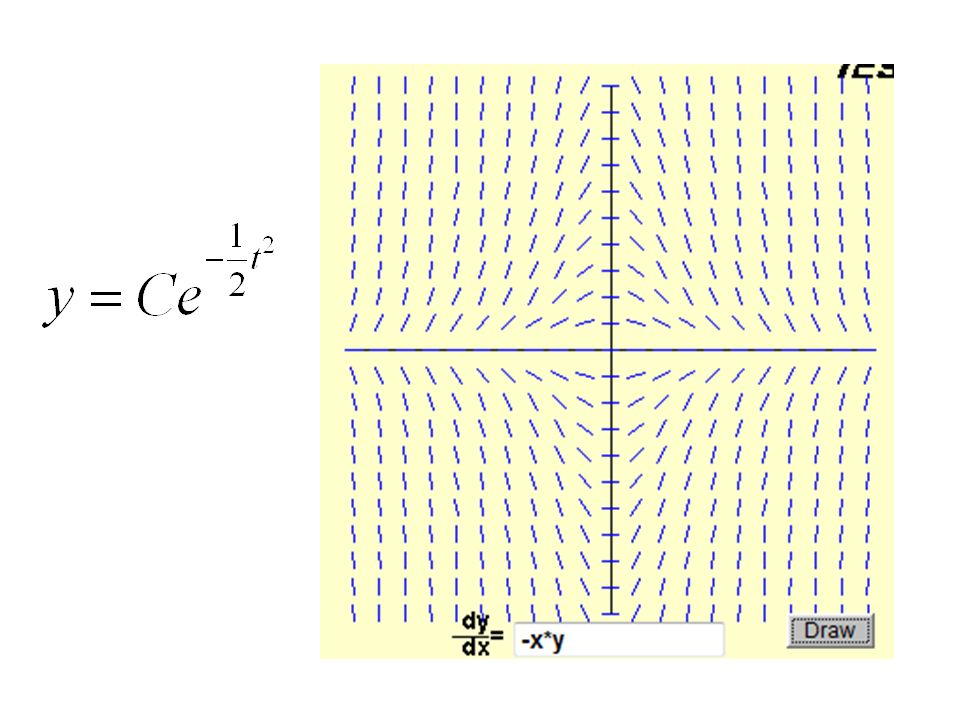
This solution would provide us with the following slope field. With each red curve being a particular solution of the form

7
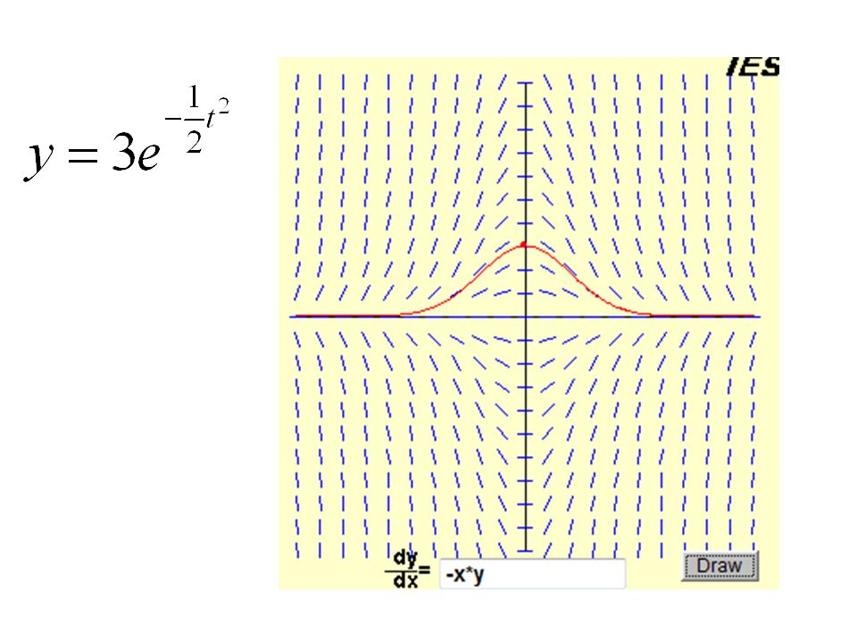
In physical situations it is more useful to identify one particular solution. In order to do this we need initial conditions. Solve the initial value problem y’=-ty with y(0)=3.
=3..")
8
y’=-ty

9
EXPONENT RULES Absolute value Because e c is a constant we can assume that it is either an arbitrary positive constant or and arbitrary negative constant, therefore we can neglect the ±. Also because e c is a constant lets re-write it as just C. So this becomes our general solution, now lets find the particular solution knowing y(0)=3 Substitute for y and t, and solve for C.
=3 Substitute for y and t, and solve for C..")
11
The particular solution is then

13
Multiply to get the numerator to the other side Apply the tangent sum formula to simplify more.

14
Rogawski text

18
Finding a Particular Solution Given the initial condition y(0)=1 find the particular solution of the equation. Rogawski text

19
Homogenous Differential Equations Homogenous means “of the same degree” – Basically we want to look at each term and determine that throughout the entire equation each term has the same degree. If it is xy, then add the exponents and you get degree 2. Homogenous equations can be transformed with substitution (y=vx) and then once that substitution is made, the equation will become separable.
 and then once that substitution is made, the equation will become separable..")
20
Determining the degree of homogenous equations. Sometimes you can simply just look at the exponents and make sure that they are all the same, (easy if everything is multiplication/addition/subtraction). The difficult part is when the equations are rational (fractions).
. The difficult part is when the equations are rational (fractions)..")
21
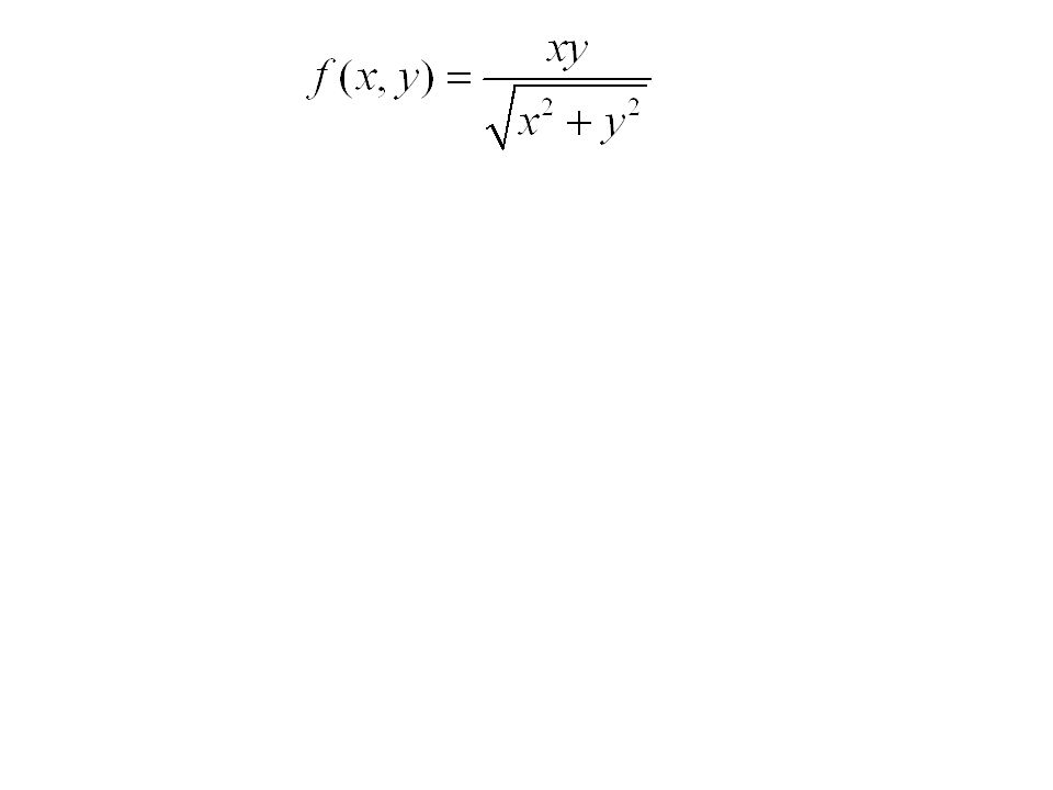
What happens when you cannot just count them? Replace every x with tx, replace every y with ty. Do the algebra to simplify the expression and try to factor out all the t’s. If you are left with t n * the original function. If this is the case, then n tells you what degree the homogenous equation is.

22
The book talks about it like this. If you start off with f(x,y) “a function with both x and y in it” Then if f(tx,ty) = t n f(x,y) then the function is homogenous of degree n.
 a function with both x and y in it Then if f(tx,ty) = t n f(x,y) then the function is homogenous of degree n..")
23
Homogenous degree 2

24
Homogenous degree 3

25
Not homogenous

27
Now that we know how to determine if an equation is homogenous or not, the authors of the book are assuming that we can go through the steps in making that determination so in the next few examples we are going to assume that we have already determined that the equations provided are homogenous (we may have to determine a degree first however, depending on what method we want to use). If we were to approach a DE and it was not separable, we would take the steps of using f(tx,ty) to determine if it was homogenous and then take the steps that involves substitution to force that homogenous equation to become separable.
 to determine if it was homogenous and then take the steps that involves substitution to force that homogenous equation to become separable..")
28
When we use this change of variables technique, we want to use y=vx. But we are also going to need the derivative of the equation y=vx, so we will use implicit differentiation to the equation y=vx.

Similar presentations


 If u and v are differentiable functions, then ∫ u dv = uv – ∫ v du. There are two ways to integrate by parts; the.>")


