1. Empirical Efficiency Maximization: Locally Efficient Covariate Adjustment in Randomized Experiments Daniel B. Rubin Joint work with Mark J. van der Laan

2. Outline Review adjustment in experiments. Locally efficient estimation. Problems with standard methods. New method addressing problems. Abstract formulation. Back to experiments, with simulations and numerical results. Application to survival analysis.

3. Randomized Experiments (no covariates yet)

4. Randomized Experiments

5. Example: Women recruited. Randomly assigned to diaphragm or no diaphragm. See if they get HIV. Example: Men recruited. Randomly assigned to circumcision or no circumcision. See if they get HIV.

6. Randomized Experiments Randomization allows causal inference. No confounding. Differences in outcomes between treatment and control groups are due to the treatment. Unverifiable assumptions needed for causal inference in observational studies.

7. Counterfactual Outcome Framework: Neyman-Rubin Model

8. Causal Parameters

9. Causal Parameters (binary response)

10. Estimating Causal Parameters in Randomized Experiments

11. Randomized Experiments with Covariates Same setup, only now demographic or clinical measurements taken prior to randomization. Question: With extra information, can we more precisely estimate causal parameters? Answer: Yes. (Fisher, 1932). Subject’s covariate has information about how he or she would have responded in both arms.

12. Covariate Adjustment (has at least two meanings) 1: Gaining precision in randomized experiments. 2: Accounting for confounding in observational studies. This talk only deals with the first meaning.

13. Covariate Adjustment. Not very difficult when covariates divide subjects into a handful of strata. Have to think with a single continuous covariate (e.g. age). Modern studies can collect a lot of baseline information. Gene expression profile, complete medical history, biometric measurements. Important longstanding problem, but lots of confusion. Not “solved.” Recent work by others.

14. Covariate Adjustment Pocock et al. (2002) recently surveyed 50 clinical trial reports. Of 50 reports, 36 used covariate adjustment for estimating causal parameters, and 12 emphasized adjusted over unadjusted analysis. “Nevertheless, the statistical emphasis on covariate adjustment is quite complex and often poorly understood, and there remains confusion as to what is an appropriate statistical strategy.”

15. Recent Work on this Problem Koch et al. (1998). - Modifications to ANCOVA. Tsiatis et al. (2000, 2007a, 2007b). - Locally efficient estimation. Moore and van der Laan (2007). - Targeted maximum likelihood. Freedman (2007a, 2007b). - Classical methods under misspecification.

16. Covariate Adjustment Can choose to ignore baseline measurements. Why might extra precision be worth it? Narrow confidence intervals for treatment effect. Stop trials earlier. Subgroup analysis, having smaller sample sizes.

17. Covariate Adjustment

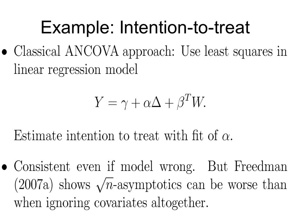
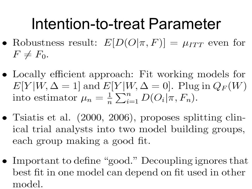
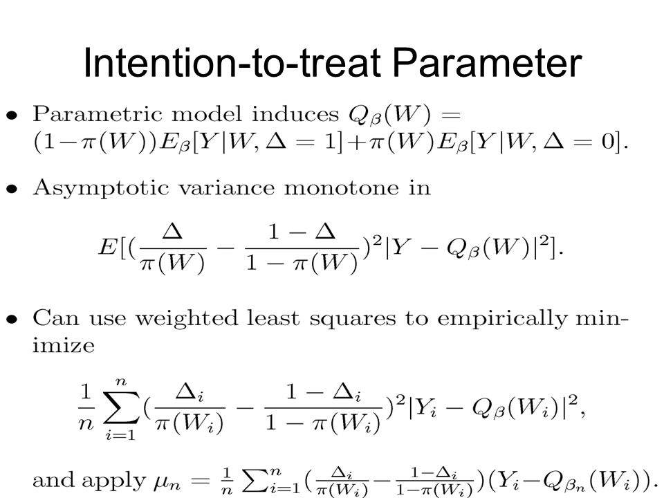
18. Example: Intention-to-treat

20. Example: Log Odds Ratio

21. Locally Efficient Estimation Primarily motivated by causal inference problems in observational studies. Origin in Robins and Rotnitzky (1992), Robins, Rotnitzky, and Zhao (1994). Surveyed in van der Laan and Robins (2003), Tsiatis (2006).

22. Locally Efficient Estimation

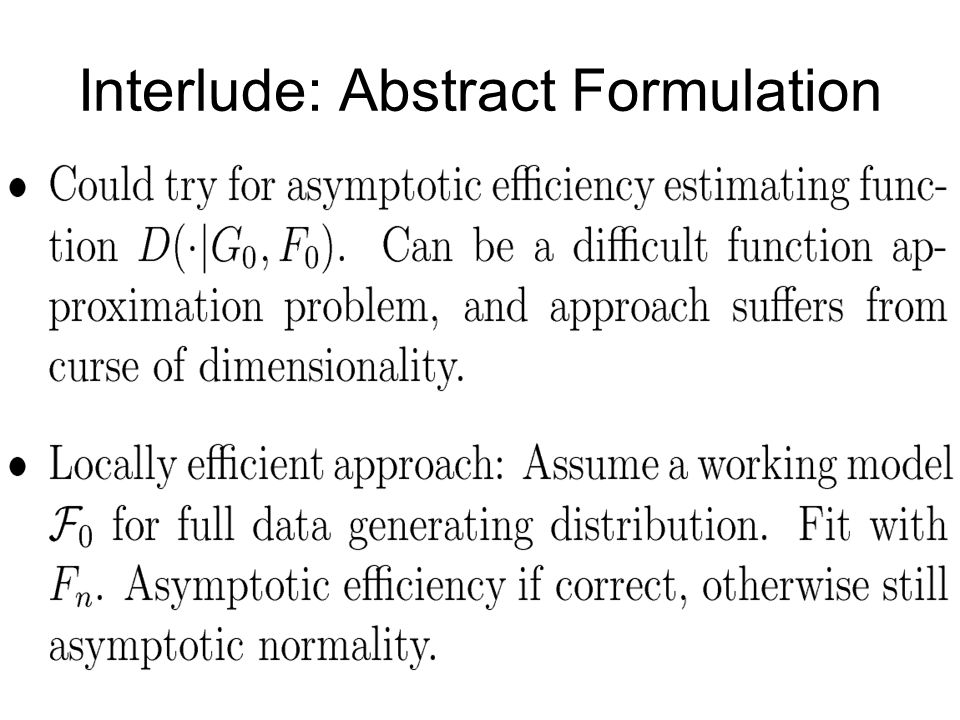
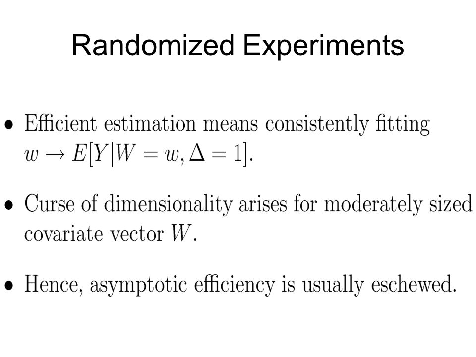
23. Locally Efficient Estimation in Randomized Experiments Working model for treatment distribution given covariates known by design. So what does local efficiency tell us? Model outcome distribution given (covariates, treatment). We’ll be asymptotically efficient if working model is correct, but still asymptotically normal otherwise. But what does this mean if there’s no reason to believe the working model? Unadjusted estimators are also asymptotically normal. What about precision?

24. Empirical Efficiency Maximization Working model for outcome distribution given (treatment, covariates) typically fit with likelihood-based methods. Often linear, logistic, or Cox regression models. “Factorization of likelihood” means such estimates lead to double robustness in observational studies. But such robustness is superfluous in controlled experiments. We try to find the working model element resulting in the parameter estimate with smallest asymptotic variance.

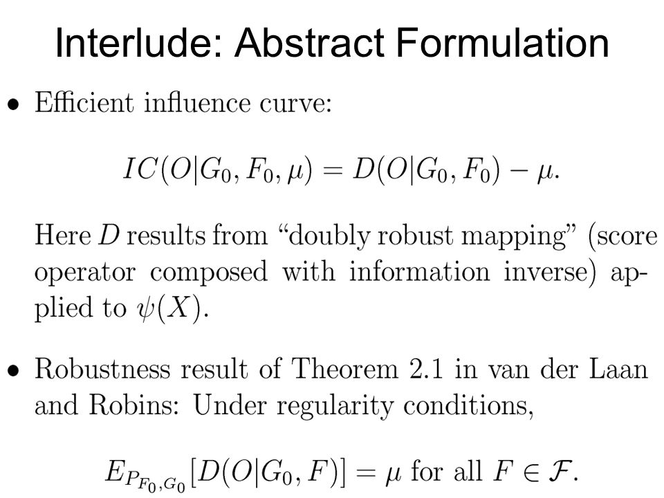
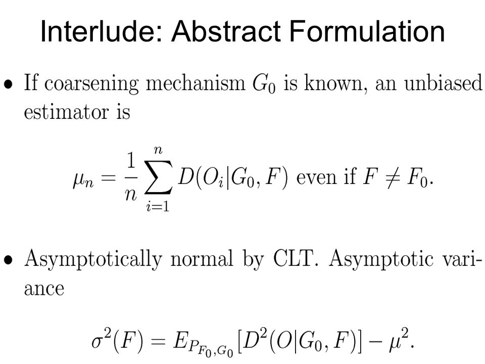
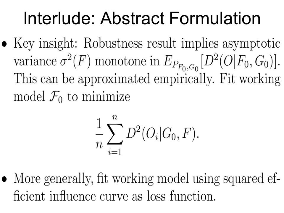
25. Interlude: Abstract Formulation

30. Asymptotics

31. Interlude: Abstract Formulation

32. Back to Randomized Experiments

33. Randomized Experiments

35. Working Model Loss Function

36. Connection to High Dimensional or Complex Data Suppose a high dimensional covariate is related to the outcome, and we would like to adjust for it to gain precision. Many steps in data processing can be somewhat arbitrary (e.g. dimension reduction, smoothing, noise removal). With cross-validation, new loss function can guide selection of tuning parameters governing this data processing.

37. Numerical Asymptotic Efficiency Calculations

38. 1=Unadjusted estimator ignoring covariates. 2=Likelihood-based locally efficient. 3=Empirical efficiency maximization. 4=Efficient.

39. Intention-to-treat Parameter

42. Numerical Asymptotic Efficiency Calculations

43. 1=Unadjusted difference in means. 2=Standard likelihood-based locally efficient estimator. 3=empirical efficiency maximization. 4=efficient estimator.

44. Treatment Effects

45. Sneak Peak: Survival Analysis

46. Form locally efficient estimate. Working model for full data distribution now likely a proportional hazards model. For estimating (e.g. five-year survival), will be asymptotically efficient if model correct. Otherwise still asymptotically normal. But locally efficient estimator can be worse than Kaplan-Meier if model is wrong.

47. Sneak Peak: Survival Analysis

48. Sneak Peak: Survival Analysis. Generated Data. Want five-year survival.

49. 1=Kaplan-Meier. 2=Likelihood-based locally efficient. 3=Empirical efficiency maximization. 4=Efficient.

50. Summary Robins and Rotnitzky’s locally efficient estimation developed for causal inference in observational studies. In experiments, estimators can gain or lose efficiency, depending on validity of working model. Often there might be no reason to have any credence in a working model. A robustness result implies we can better fit working model (or select tuning parameters in data processing) with a nonstandard loss function (the squared influence curve).

51. Troublesome Issues When working regression model is linear, our procedure usually reduces to existing procedures. When nonlinear, fitting regression model with our loss function can entail non- convex optimization. Proving convergence to working model elements for well-known logistic and Cox regression models.

52. References Empirical Efficiency Maximization: Improved Locally Efficient Covariate Adjustment. In press in International Journal of Biostatistics. Technical reports at www.bepress.com/ucbbiostat/paper229/ and www.bepress.com/ucbbiostat/paper220/. www.bepress.com/ucbbiostat/paper229/ www.bepress.com/ucbbiostat/paper220/