1. Nonparametric Statistics

2. In previous testing, we assumed that our samples were drawn from normally distributed populations. This chapter introduces some techniques that do not make that assumption. These methods are called distribution-free or nonparametric tests. In situations where the normal assumption is appropriate, nonparametric tests are less efficient than traditional parametric methods. Nonparametric tests frequently make use only of the order of the observations and not the actual values.

3. In this section, we will discuss four nonparametric tests: the Wilcoxon Rank Sum Test (or Mann-Whitney U test), the Wilcoxon Signed Ranks Test, the Kruskal-Wallis Test, and the one sample test of runs.

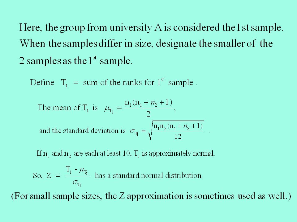
4. The Wilcoxon Rank Sum Test or Mann-Whitney U Test This test is used to test whether 2 independent samples have been drawn from populations with the same median. It is a nonparametric substitute for the t-test on the difference between two means.

5. Based on the following samples from two universities, test at the 10% level whether graduates from the two schools have the same average grade on an aptitude test. Wilcoxon Rank Sum Test Example: university AB 5070 5273 5677 6080 6483 6885 7187 7488 8996 9599

6. university AB 5070 5273 5677 6080 6483 6885 7187 7488 8996 9599 First merge and rank the grades. Sum the ranks for each sample. rankgradeuniversity 150A 252A 356A 460A 564A 668A 770B 871A 973B 1074A 1177B 1280B 1383B 1485B 1587B 1688B 1789A 1895A 1996B 2099B rank sum for university A: 74 rank sum for university B: 136 Note: If there are ties, each value gets the average rank. For example, if 2 values tie for 3 th and 4 th place, both are ranked 3.5. If three differences would be ranked 7, 8, and 9, rank them all 8.

8. -1.645 0 1.645Z.45.05 critical region Since the critical values for a 2-tailed Z test at the 10% level are 1.645 and -1.645, we reject H 0 that the medians are the same and accept H 1 that the medians are different.

9. For small sample sizes, you can use Table E.6 in your textbook, which provides the lower and upper critical values for the Wilcoxon Rank Sum Test. That table shows that for our 10% 2-tailed test, the lower critical value is 82 and the upper critical value is 128. Since our smaller sample’s rank sum is 74, which is outside the interval (82, 128) indicated in the table, we reject the null hypothesis that the medians are the same and conclude that they are different. Equivalently, since the larger sample’s rank sum is 136, which is also outside the interval (82, 128), we again reject the null hypothesis that the medians are the same and conclude that they are different.

10. The Wilcoxon Signed Rank Test This test is used to test whether 2 dependent samples have been drawn from populations with the same median. It is a nonparametric substitute for the paired t-test on the difference between two means.

11. Wilcoxon Signed Rank Test Procedure 1.Calculate the differences in the paired values (D i =X 1i – X 2i ) 2.Take absolute values of the differences and rank them (Discard all differences that equal 0.) 3.Assign ranks R i with the smallest rank equal to 1. As in the rank sum test, if two or more of the differences are equal, each difference gets the average rank. (That is, if two differences would be ranked 3 and 4, rank them both 3.5. If three differences would be ranked 7, 8, and 9, rank them all 8.) 4.Assign the symbol + to positive differences and – to negative differences. 5.Calculate the Wilcoxon statistic W as the sum of the positive ranks. So,

12. Wilcoxon Signed Rank Test Procedure (cont’d)

13. exam1exam2 diff (ex2-ex1) rank (+) rank (-) exam1exam2 diff (ex2-ex1) rank (+) rank (-) 95977268 76 7894 82755855 48547375 27317170 34396966 58615762 98978492 45 9181 77948390 27366773 Example Suppose we have a class with 22 students, each of whom has two exam grades. We want to test at the 5% level whether there is a difference in the median grade for the two exams.

14. exam1exam2 diff (ex2-ex1) rank (+) rank (-) exam1exam2 diff (ex2-ex1) rank (+) rank (-) 959727268-4 76 0789416 8275-75855-3 4854673752 273147170 343956966-3 5861357625 989784928 45 09181-10 77941783907 2736967736 We calculate the difference between the exam grades: diff = exam2 – exam 1.

15. exam1exam2 diff (ex2-ex1) rank (+) rank (-) exam1exam2 diff (ex2-ex1) rank (+) rank (-) 959727268-4 76 0789416 8275-75855-3 4854673752 2731471701.5 343956966-3 5861357625 98971.584928 45 09181-10 77941783907 2736967736 Then we rank the absolute values of the differences from smallest to largest, omitting the two zero differences. The smallest non-zero |differences| are the two |-1|’s. Since they are tied for ranks 1 and 2, we rank them both 1.5. Since the differences were negative, we put the ranks in the negative column.

16. exam1exam2 diff (ex2-ex1) rank (+) rank (-) exam1exam2 diff (ex2-ex1) rank (+) rank (-) 959723.57268-4 76 0789416 8275-75855-3 48546737523.5 2731471701.5 343956966-3 5861357625 98971.584928 45 09181-10 77941783907 2736967736 The next smallest non-zero |differences| are the two |2|’s. Since they are tied for ranks 3 and 4, we rank them both 3.5. Since the differences were positive, we put the ranks in the positive column.

17. exam1exam2 diff (ex2-ex1) rank (+) rank (-) exam1exam2 diff (ex2-ex1) rank (+) rank (-) 959723.57268-4 76 0789416 8275-75855-36 48546737523.5 2731471701.5 343956966-36 58613657625 98971.584928 45 09181-10 77941783907 2736967736 The next smallest non-zero |differences| are the two |-3|’s and the |3|. Since they are tied for ranks 5, 6, and 7, we rank them all 6. Then we put the ranks in the appropriately signed columns.

18. exam1exam2 diff (ex2-ex1) rank (+) rank (-) exam1exam2 diff (ex2-ex1) rank (+) rank (-) 95972 3.5 7268-4 8.5 76 0789416 19 8275-7 14.5 5855-3 6 48546 12.5 73752 3.5 27314 8.5 7170 1.5 34395 10.5 6966-3 6 58613 6 57625 10.5 9897 1.5 84928 16 45 09181-10 18 779417 20 83907 14.5 27369 17 67736 12.5 We continue until we have ranked all the non-zero |differences|.

19. exam1exam2 diff (ex2-ex1) rank (+) rank (-) exam1exam2 diff (ex2-ex1) rank (+) rank (-) 95972 3.5 7268-4 8.5 76 0789416 19 8275-7 14.5 5855-3 6 48546 12.5 73752 3.5 27314 8.5 7170 1.5 34395 10.5 6966-3 6 58613 6 57625 10.5 9897 1.5 84928 16 45 09181-10 18 779417 20 83907 14.5 27369 17 67736 12.5 15456 Then we total the signed ranks. We get 154 for the sum of the positive ranks and 56 for the sum of the negative ranks. The Wilcoxon test statistic is the sum of the positive ranks. So W = 154.

20. Since we had 22 students and 2 zero differences, the number of non-zero differences n = 20. -1.96 0 1.96Z.475.025 critical region Since the critical values for a 2-tailed Z test at the 5% level are 1.96 and -1.96, we can not reject the null hypothesis H 0 and so we conclude that the medians are the same.

21. For small sample sizes, you can use Table 12.19 in the online material associated with section 12.8 of your textbook, which provides the lower and upper critical values for the Wilcoxon Signed Rank Test. This table is shown on the next slide.

22. Lower & Upper Critical Values, W, of Wilcoxon Signed Ranks Test ONE-TAILα = 0.05α = 0.025α = 0.01α = 0.005 TWO-TAILα = 0.10α = 0.05α = 0.02α = 0.01 n(Lower, Upper) 50,15—,— 62,190,21—,— 73,252,260,28—,— 85,313,331,350,36 98,375,403,421,44 1010,458,475,503,52 1113,5310,567,595,61 1217,6113,6510,687,71 1321,7017,7412,7910,81 1425,8021,8416,8913,92 1530,9025,9519,10116,104 1635,10129,10723,11319,117 1741,11234,11927,12623,130 1847,12440,13132,13927,144 1953,13746,14437,15332,158 2060,15052,15843,16737,173 Recall that we have 20 non-zero differences and are performing a 5% 2-tailed test. Here we see that the lower critical value is 52 and the upper critical value is 158. Our statistic W, the sum of the positive ranks, is 154, which is inside the interval (52, 158) indicated in the table. So we can not reject the null hypothesis and we conclude that the medians are the same.

23. The Kruskal-Wallis Test This test is used to test whether several populations have the same median. It is a nonparametric substitute for a one-factor ANOVA F-test.

24. where n j is the number of observations in the j th sample, n is the total number of observations, and R j is the sum of ranks for the j th sample. In the case of ties, a corrected statistic should be computed: where t j is the number of ties in the j th sample.

25. Kruskal-Wallis Test Example: Test at the 5% level whether average employee performance is the same at 3 firms, using the following standardized test scores for 20 employees. Firm 1Firm 2Firm 3 scorerankscorerankscorerank 786882 957765 858450 876193 756270 907260 8073 n 1 = 7n 2 = 6n 3 =7

26. We rank all the scores. Then we sum the ranks for each firm. Then we calculate the K statistic. Firm 1Firm 2Firm 3 scorerankscorerankscorerank 78126868214 95207711655 85168415501 87176139319 7510624707 9018728602 8013739 n 1 = 7R 1 = 106n 2 = 6R 2 = 47n 3 =7R 3 = 57

27. f(  2 ) acceptance region crit. reg..05 5.991 From the  2 table, we see that the 5% critical value for a  2 with 2 dof is 5.991. Since our value for K was 6.641, we reject H 0 that the medians are the same and accept H 1 that the medians are different.

28. One sample test of runs a test for randomness of order of occurrence

29. A run is a sequence of identical occurrences that are followed and preceded by different occurrences. Example: The list of X’s & O’s below consists of 7 runs. x x x o o o o x x o o o o x x x x o o x

30. Suppose r is the number of runs, n 1 is the number of type 1 occurrences and n 2 is the number of type 2 occurrences.

31. If n 1 and n 2 are each at least 10, then r is approximately normal.

32. Example: A stock exhibits the following price increase (+) and decrease (  ) behavior over 25 business days. Test at the 1% whether the pattern is random. + + +   +    + +  +  +   + +  + +  +  r =16, n 1 (+) = 13, n 2 (  ) = 12 Since the critical values for a 2-tailed 1% test are 2.575 and -2.575, we accept H 0 that the pattern is random. -2.575 0 2.575 Z critical region.005 acceptance region.495