Download presentation
Presentation is loading. Please wait.

1
Learning Time-Series Shapelets Josif Grabocka, Nicolas Schilling, Martin Wistuba, Lars Schmidt-Thieme Information Systems and Machine Learning Lab University of Hildesheim 14’ SIGKDD

2
Outline Introduction Related Work Proposed Method Analysis of The Proposed Method Learning General Shapelets Experimental Results Conclusion and Comments

3
Outline Introduction Related Work Proposed Method Analysis of The Proposed Method Learning General Shapelets Experimental Results Conclusion and Comments

4
Shapelet 0 200400600800100012001400 Figure 1: left) Skulls of horned lizards and turtles. right) the time series representing the images. The 2D shapes are converted to time series using the technique in [14]
 the time series representing the images. The 2D shapes are converted to time series using the technique in [14].")
5
Shapelet Figure 2: left) The shapelet that best distinguishes between skulls of horned lizards and turtles, shown as the purple/bold subsequence. right) The shapelet projected back to the original 2D shape space
 The shapelet projected back to the original 2D shape space.")
6
Shapelet Orderline 0 ∞ split candidate Figure 3: The orderline shows the distance between the candidate subsequence and all time series as positions on the x-axis. The three objects on the left hand side of the line correspond to horned lizards and the three objects on the right correspond to turtles

7
SOTA Shapelet Mining Method State-of-the-art methods discover shapelets by trying a pool of candidate sub-sequences from all possible series segments and then sorting the top performing segments according to their target prediction qualities. A method called Shapelet-transformation has recently shown improvements with respect to prediction accuracy.

8
The Proposed Method This work proposes a mathematical formulation of the shapelet learning task as an optimization of a classification objective function. Furthermore, this work proposes a method that learns (not searches for) the shapelets which optimize the objective function. Concretely, the proposed method learns shapelets whose distances to series can linearly separate the time series instances by their targets. In comparison to existing approaches, this method can learn near-to- optimal shapelets and true top-K shapelet interactions.
 the shapelets which optimize the objective function. Concretely, the proposed method learns shapelets whose distances to series can linearly separate the time series instances by their targets. In comparison to existing approaches, this method can learn near-to- optimal shapelets and true top-K shapelet interactions..")
9
The Proposed Method

10
Outline Introduction Related Work Proposed Method Analysis of The Proposed Method Learning General Shapelets Experimental Results Conclusion and Comments

11
Original Concept, Quality Metrics and Shapelet Transformation Shapelets were first proposed as time-series segments that maximally predict the target variable. All possible segments were considered as potential candidates, while the minimum distances of a candidate to all training series were used as a predictor feature for ranking the information gain accuracy of that candidate on the target variable. Other quality measures include F-Stats, Kruskal-Wallis and Mood’s median. Standard classifiers have achieved high accuracy over the shapelet- transformed representation.

12
Speed-up Techniques Early abandoning of distance computations. Entropy pruning of the information gain metric. Reuse of computations. Pruning of the search space. Exploiting projections on the SAX representation. Elaborating the usage of infrequent shapelet candidates. Hardware-based optimization assisted shapelet discovery using GPUS.

13
Real-life Applications Clustering time series using unsupervised shapelets. Identifying human through their gait data. Gesture recognition. Early classification of medical and health informatics related time series.

14
Outline Introduction Related Work Proposed Method Analysis of The Proposed Method Learning General Shapelets Experimental Results Conclusion and Comments

15
Key Techniques Shapelet Transformation Logistic Regression Stochastic Gradient Descent K-Means Clustering

16
Definitions and Notations Time Series Dataset: A time-series dataset composed of I training instances, with each series contains Q-many ordered values, is denoted as T I× Q, while the series target is a nominal variable Y ∈ {1,..., C} I having C categories. *The proposed method can operate on variable series lengths. Sliding Window Segment: A sliding window segment of length L is an ordered sub-sequence of a series. Concretely, the segment starting at time j inside the i-th series is defined as (T i,j,..., T i,j+L−1 ). There are totally J := Q − L + 1 segments in a time series provided the starting index of the sliding window is incremented by one.
. There are totally J := Q − L + 1 segments in a time series provided the starting index of the sliding window is incremented by one..")
17
Definitions and Notations

18
Go to Differentiable Soft-Minimum Function.

19
Definitions and Notations Go to Objective Function: Learning Model.

20
Definitions and Notations

21
Learning Model Go to Differentiable Soft-Minimum Function.

22
Loss Function

23
Regularized Objective Function Go to Per-Instance Objective.

24
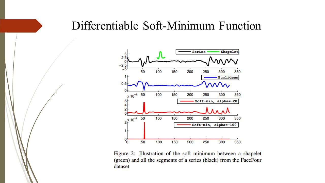
Differentiable Soft-Minimum Function

25
Go to Differentiable Soft-Minimum Function.

26
Differentiable Soft-Minimum Function

29
Per-Instance Objective

30
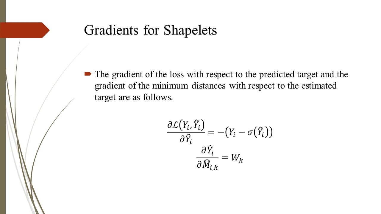
Gradients for Shapelets

32
Gradients Shapelets

33
Gradients for Shapelets

34
Gradients for Weights

35
Optimization Algorithm

36
Convergence The convergence of the optimization algorithm depends on two parameters, the learning rate η and the maximum number of iterations. To determine the optimal values of these two parameters, this work implements cross-validation.

37
Convergence

38
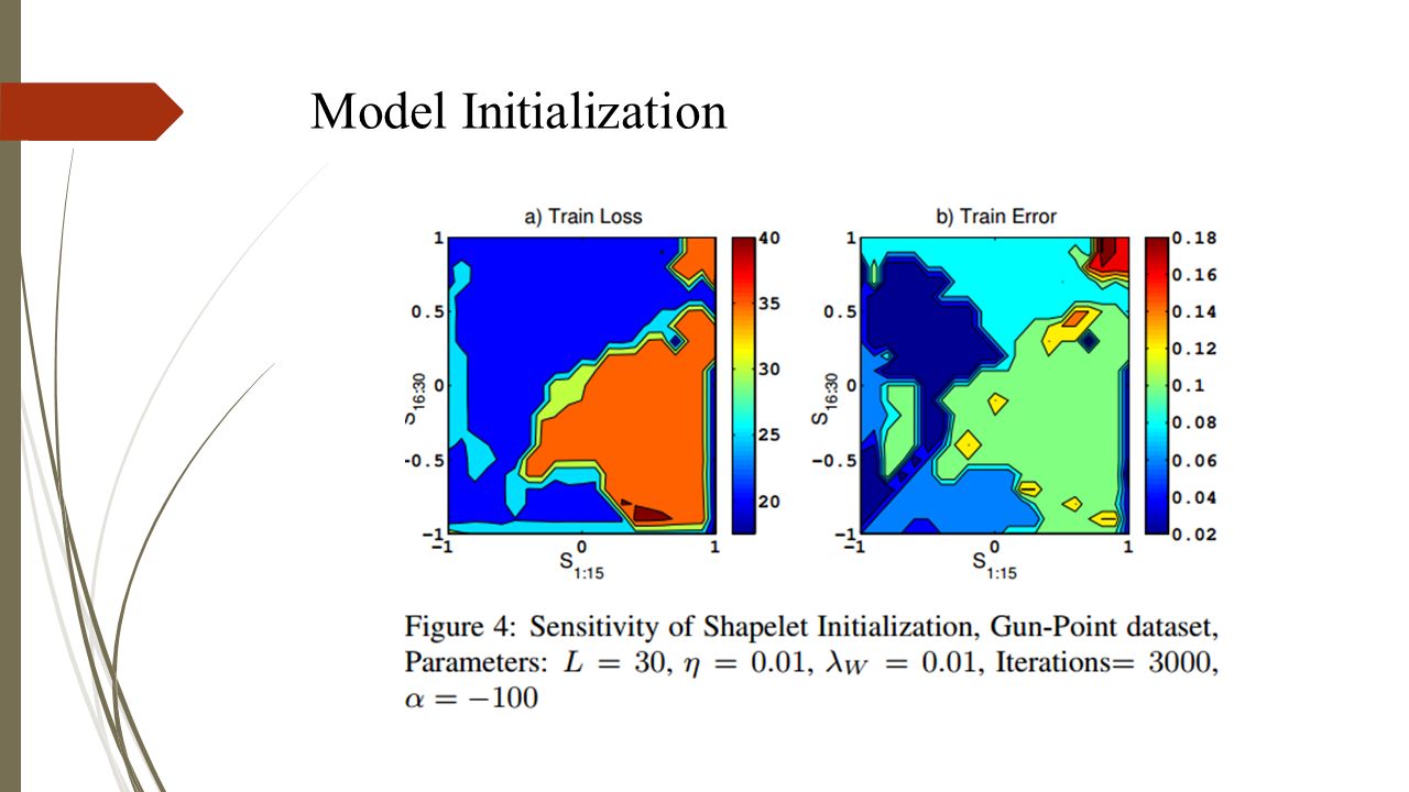
Model Initialization

40
If the initialization starts the learning around a region where the global optimum is located, then the gradient can update the parameters to the exact location of the optimum. In order to robustify the initialization guesses, this work uses the K- Means centroids of all segments as initial values for the shapelets. Since centroids represent typical patterns of the data, they offer a good variety of shapes for initializing shapelets and help our method achieve high prediction accuracy. The hyper-plane W is also initialized randomly around 0.

41
Illustrating The Mechanism

42
Outline Introduction Related Work Proposed Method Analysis of The Proposed Method Learning General Shapelets Experimental Results Conclusion and Comments

43
Algorithmic Complexity

44
VS. SOTA: Learning Near-to-Optimal Shapelets This: The gradient descent approach can find a near-to-optimal minimum given an appropriate initialization. Baselines: No such guarantee for two primary reasons. First of all, the baselines are bound to shapelet candidates from the pool of series segments and cannot explore candidates which do not appear literally as segments. Secondly, minimizing the classification objective through candidate guesses has no guarantee of optimality.

45
VS. SOTA: Capturing Interactions Among Shapelets The baselines find the score of each shapelet independently, ignoring the interactions among patterns. In reality, two shapelets can be individually sub-optimal, but when combined together they can improve the results. This problem is well known in data mining as variable subset selection.

46
VS. SOTA: Capturing Interactions Among Shapelets

47
The baselines can address this problem by conducting an exhaustive search over all combinations of candidate shapelets, yet it is very costly and not feasible in practice. The proposed method, however, can find the interactions at a simple linear scale K, due to the property of jointly learning the shapelets and their interactions.

48
VS. SOTA: One Weaker Aspect The proposed method relies on more hyper-parameters than the baselines such as the learning rate η, the number of iterations, the regularization parameter λ W and the soft-min precision α. Nonetheless, the very high accuracy out-weights the model’s learning efforts.

49
Outline Introduction Related Work Proposed Method Analysis of The Proposed Method Learning General Shapelets Experimental Results Conclusion and Comments

50
Extending to Multi-class Cases

51
Extending to Non-fixed Shapelet Length Cases

52
Outline Introduction Related Work Proposed Method Analysis of The Proposed Method Learning General Shapelets Experimental Results Conclusion and Comments

53
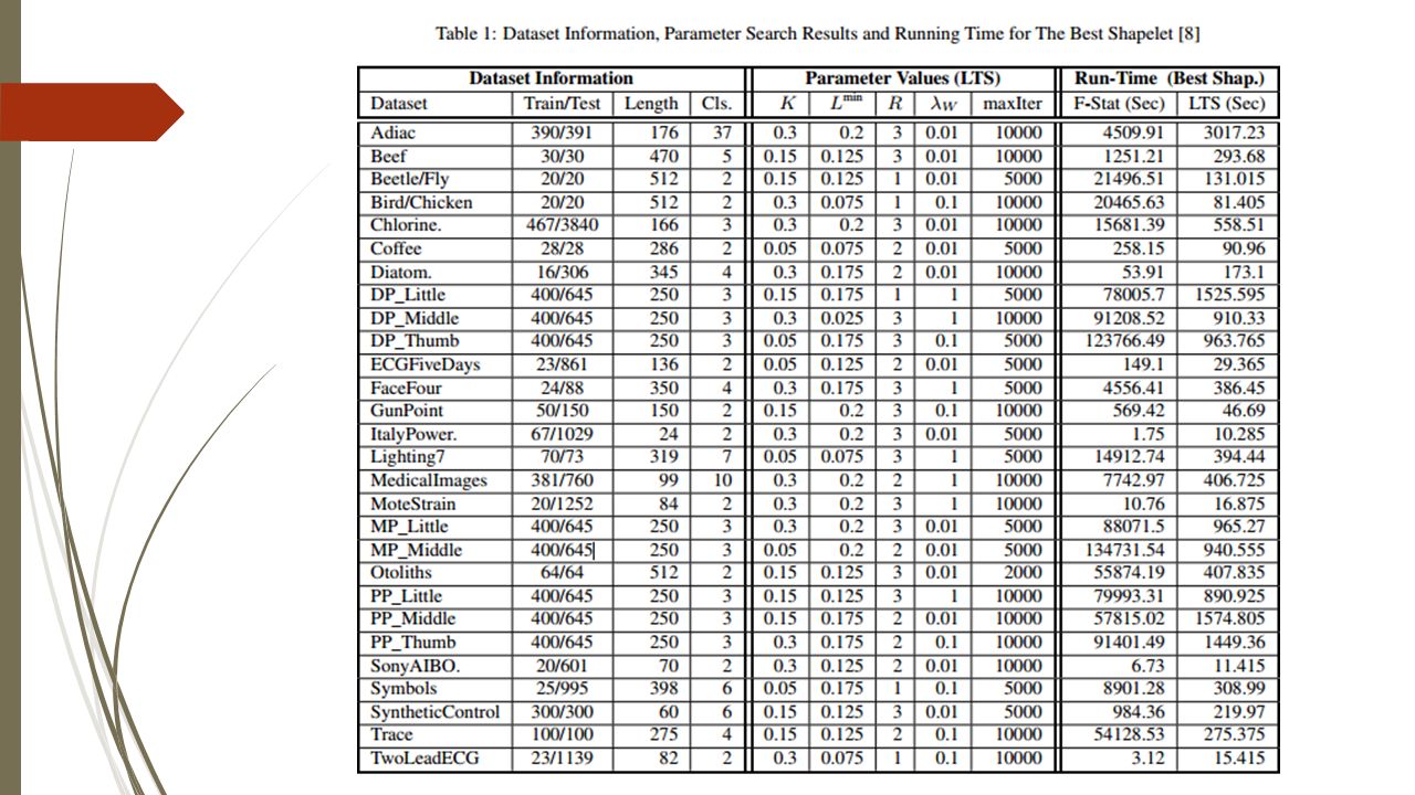
Dataset & Hyper-parameter Search

54
Baselines Shapelet Tree Methods, conducted from shapelets whose qualities are measured using: Information gain quality criterion (IG) Kruskal-Wallis quality criterion (KW) F-Stats quality criterion (FST) The Mood’s Median Criterion (MM)
 Kruskal-Wallis quality criterion (KW) F-Stats quality criterion (FST) The Mood’s Median Criterion (MM)")
55
Baselines Basic Classifiers, learned over shapelet-transformed data, such as: Nearest Neighbors (1NN) Naïve Bayes (NB) C4.5 tree (C4.5)
 Naïve Bayes (NB) C4.5 tree (C4.5)")
56
Baselines More Complex Classifiers, learned over shapelet transformed data, such as: Bayesian Networks (BN) Random Forest (RAF) Rotation Forest (ROF) Support Vector Machines (SVM)
 Random Forest (RAF) Rotation Forest (ROF) Support Vector Machines (SVM)")
57
Baselines Other Related Methods: Fast Shapelets (FSH) Dynamic Time Warping (DTW)
 Dynamic Time Warping (DTW)")
60
Outline Introduction Related Work Proposed Method Analysis of The Proposed Method Learning General Shapelets Experimental Results Conclusion and Comments

61
Conclusion and Comments Learning, not searching for, shapelets. Classic machine learning techniques. Pros: Very high accuracy. Competitive running time. Cons: Painstaking Hyper-parameter Tuning. Inadequate Interpretability.

Similar presentations


 Dealing with Indefinite Representations in Pattern Recognition.>")
>")


>")


