1. PHASE REFERENCED MAPPING AND DIFFERENTIAL ASTROMETRY: APPLICATIONS JON MARCAIDE 26 Sept 2001 Castel San Pietro Terme

2. Very Long Baseline Interferometry (VLBI) B s   = B·s / c

4. Marcaide & Shapiro, Ap.J. 276, 56-59 (1984) Phase referenced map: I(x,y) =∫∫V(u,v) e -i 2  (ux + vy) du dv  V(u,v)  e-i  A-B

5. Phase-reference mapping: Differential phase:  A-B =  A-B (str) +  A-B (pos) +  A-B (ins) +  A-B (atm) Phase referenced map: I(x,y) =∫∫V(u,v) e -i 2  (ux + vy) du dv  V(u,v)  e-i  A-B

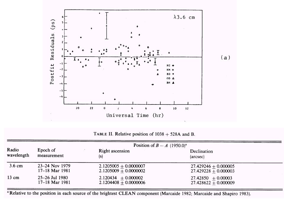
10. Marcaide & Shapiro, A.J. 88, 1134-1137 (1983)

11. Differential astrometry vs phase reference Alternating observation:  A (t 1 )  A (t 3 )  A (t 5 )  B (t 2 )  B (t 4 )  B (t 6 )... Analysis:  A (t 1 ;res) =  A (t 1 ;obs)   A (t 1 ;thr)  B (t 2 ;res) =  B (t 2 ;obs)   B (t 2 ;thr)  A-B (t’ 1 ;res) =  A (t 1 ;res)   B (t 2 ;res)  A-B (res) =  A-B (res; str) +  A-B (res; pos) +  A-B (res; ins) +  A-B (res; atm)

12. Phase-reference mapping: Differential phase:  A-B (res) =  A-B (res; str) +  A-B (res; pos) +  A-B (res; ins) +  A-B (res; atm) 0 0 Phase referenced map: I(x,y) =∫∫V(u,v) e -i 2  (ux + vy) du dv  V(u,v)  e-i  A-B(res)

13. Differential astrometry:  A-B (res) =  A-B (res; str) +  A-B (res; pos) +  A-B (res; ins) +  A-B (res; atm) 0WLSF Residuals (30º a 7mm)

14. Technique Walter Alef (1989), Very Long Baseline Interferometry: Techniques and Applications, M. Felli & R.E. Spencer, Eds. NATO ASI Series, Kluwer C283 Phil Diamond, idem Thompson, Moran & Swenson (1986) “Inteferometry and Synthesis in Radio Astronomy”, p. 384

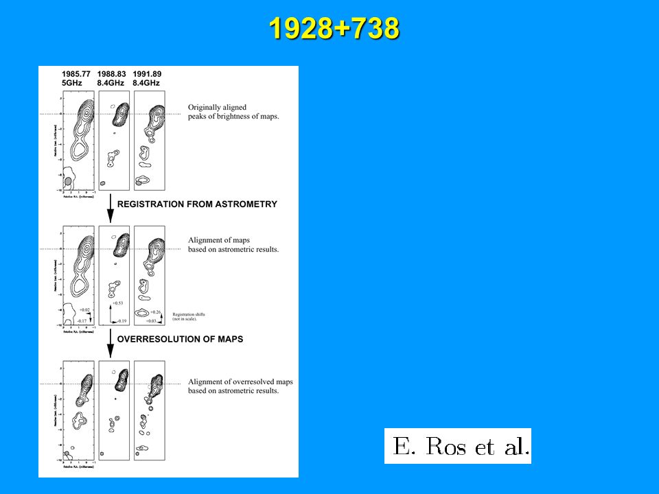
15. PRECISION DIFFERENTIAL ASTROMETRY For a long time: Standard frequencies: 8.4 & 2.3 GHz Difficulty in reference point definition: “  -arcsec astrometry vs. m-arcsec resolution images” Examples: 4C39.25, 1928+738....

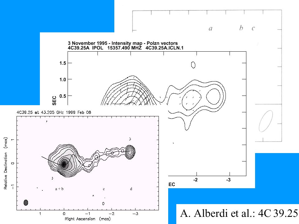
17. 4C39.25 4C39.25

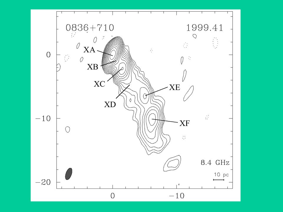
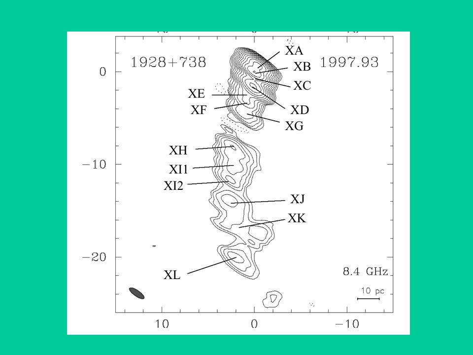
18. 1928+738 1928+738

19. A hybrid approach Observations of the pair 0735+178 / 0748+128 Combination of : 1) Differential astrometry @ 8.4 GHz 2) Simultaneous maps @ 43GHz The idea is to interpret the 8.4GHz astrometry with the help of the 43GHz maps.

20. 0735+178 0735+178 3.6cm 3.6cm

21. 0735+178 0735+178 3.6cm 3.6cm

22. 0735+178 0735+178 3.6cm 3.6cm

23. 0735+178 0735+178 3.6cm 3.6cm 7mm 7mm

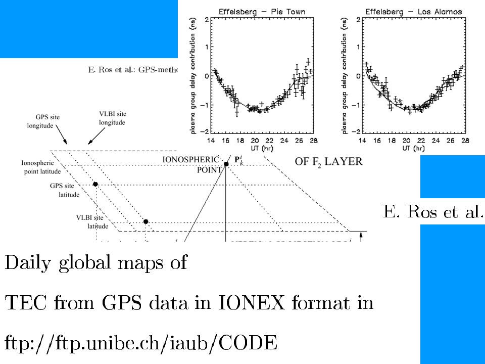
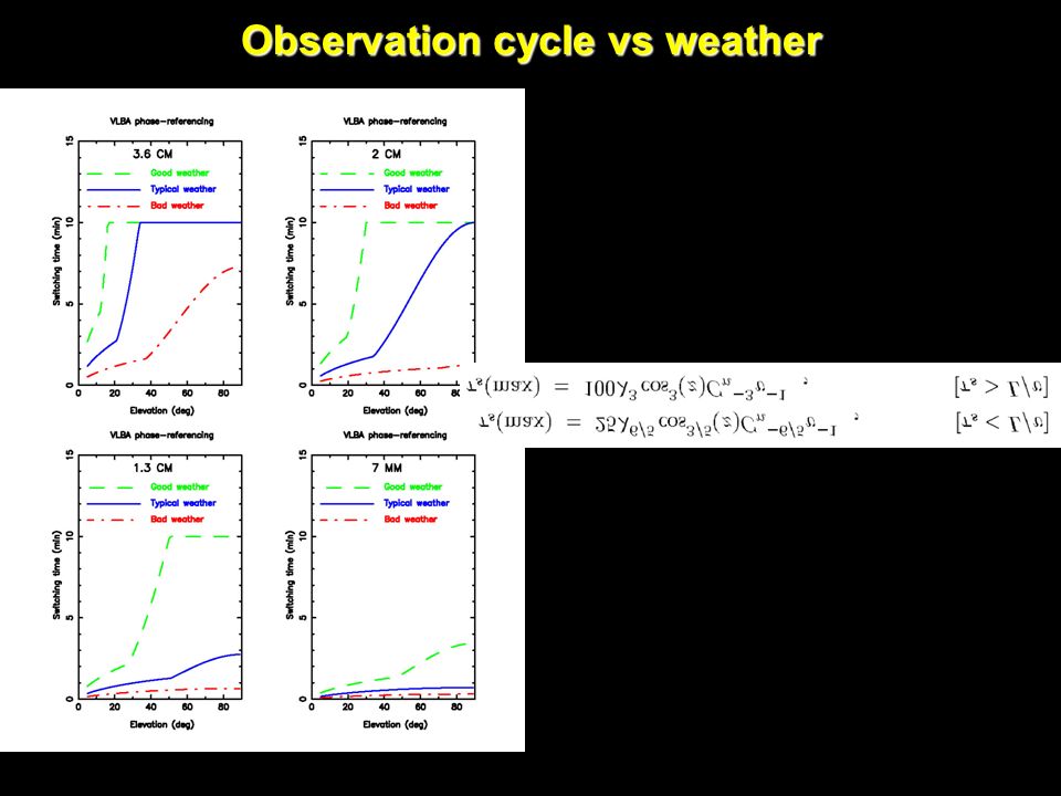
25. Differential astrometry @ 7mm Advantages: Easier identification of the reference point Reference point closer to central engine (assumed stationary) Ionospheric contribution 25 times smaller than @ 3.6cm Disadvantages: Tropospheric water vapor contribution larger Phase cycle duration: 23ps (5 times shorter than @ 3.6cm) ¿Are the Earth Orientation models precise enough to predict the interferometric phase to a small fraction of 23ps?

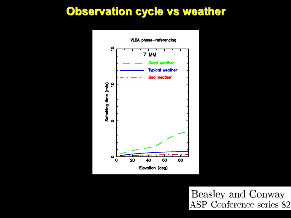
26. Astrometry @ 7mm Observation cycle vs weather Observation cycle (switching time) is VERY dependent on weather

27. Observation cycle vs weather

30. 1928+738 / 2007+777 @ 7mm 1928+738 / 2007+777 @ 7mm

31. 1928+738 / 2007+777 @ 7mm Rate residuals

32. 1928+738 / 2007+777 7mm

33. Differenced phase delay residual Differenced phase delay residual Astrometric model: IERS Standard Ionosphere (IONEX) Troposphere (nodes) r.m.s.  30º (  2 ps) Important for phase reference mapping

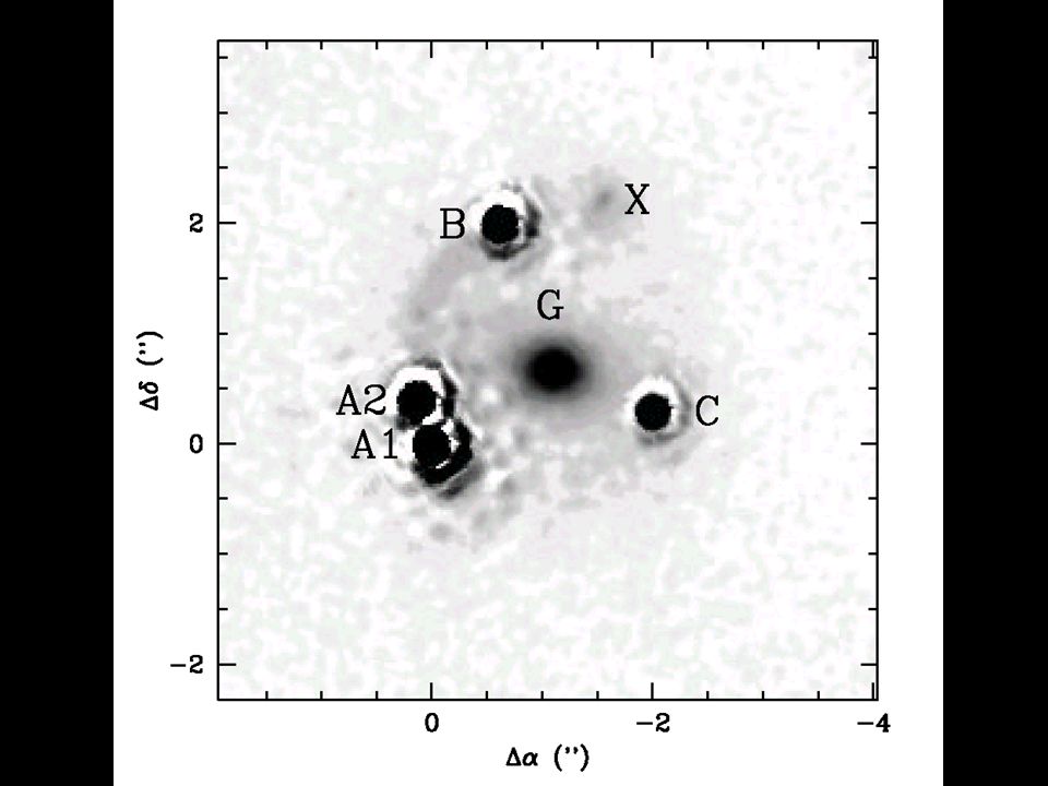
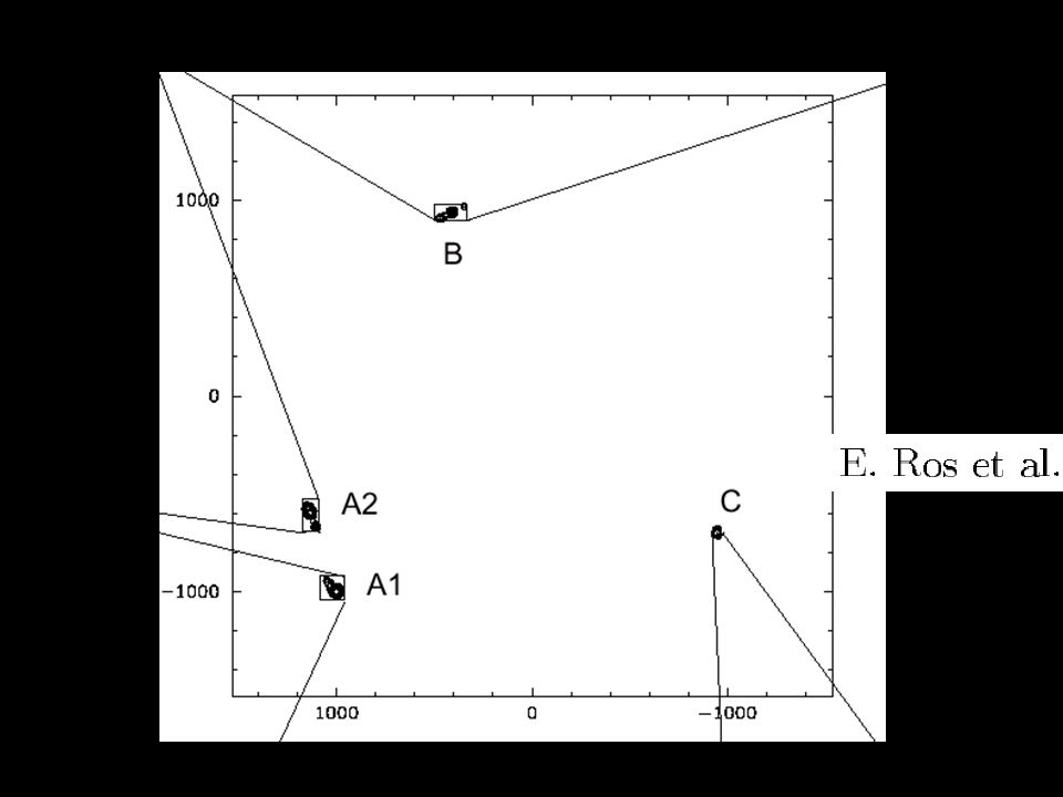
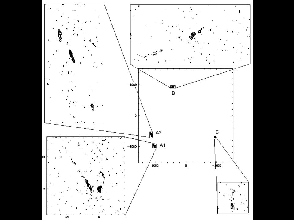
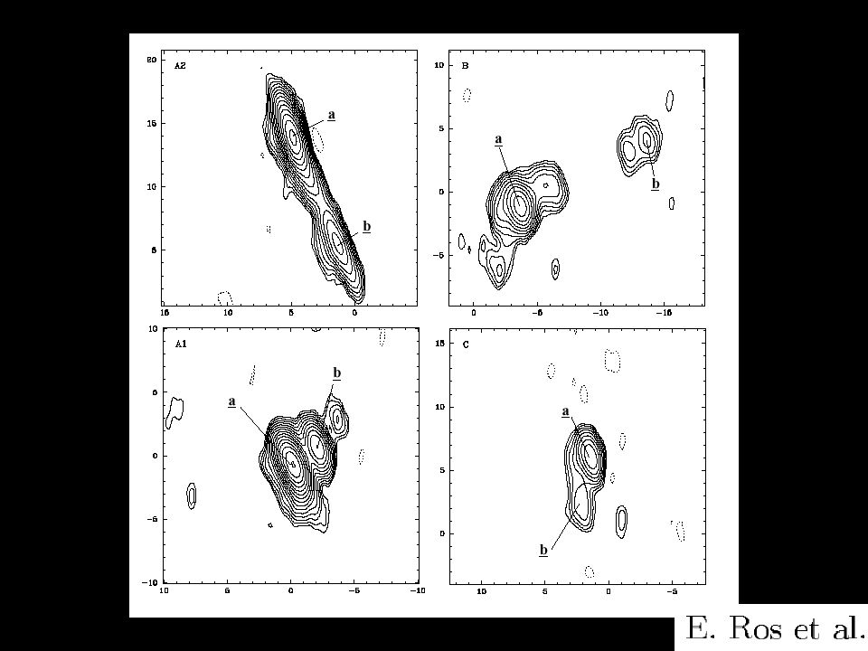
44. HST image A1 B A2 C B C A1 A2 Quadruple Gravitational Lenses: MGJ0414+0534 Ros et al., A&A (2000)

45. Beyond Earth limitations: SPACE VLBI SPACE VLBI VLBI Space Observatory Program V.S.O.P.

46. Astrometry with VSOP Halca limitations for astrometry: HALCA (Highly Advanced Laboratory for Communication and Astronomy)  Short memory span to manoever the antenna (Difficulty for alternating observations of sources)  Large fractional errors in the space baselines:  (   )     B/B  B  50-100m (JPL) This implies that for source pairs with   1º,  (   )  10 mas However, how about observing two sources simultaneously?

47. Astrometry with VSOP VLBA + HALCA observations of the pair of quasars 1342+662 / 1342+663 @ 6cm 1342+662 / 1342+663 with separation  = 4‘ have been observed simultaneously by HALCA y VLBA

48. 1342+662 / 1342+663

49. Maps of 1342+662 and 1342+663 1342+662 1342+663

50. Phase reference analysis of 1342+662 Phase reference analysis of 1342+662  A-B (res) =  A-B (res; str) +  A-B (res; pos) +  A-B (res; ins) +  A-B (res; atm) I(x,y) =∫∫V(u,v) e -i 2  (ux + vy) du dv

51. Phase reference analysis of 1342+662

52. Astrometric information:  = -0.5 mas  = 1.5 mas

53. Phases of 1342+662 referenced to 1342+663

54.  B HALCA ~ 10 m

55. Phase-referenced maps of 1342+662 VLBA +HALCA Only HALCA Only VLBA

56. Space astrometry with VSOP Scatter of position of maximum in maps : 50  as  B HALCA ~ 3 m

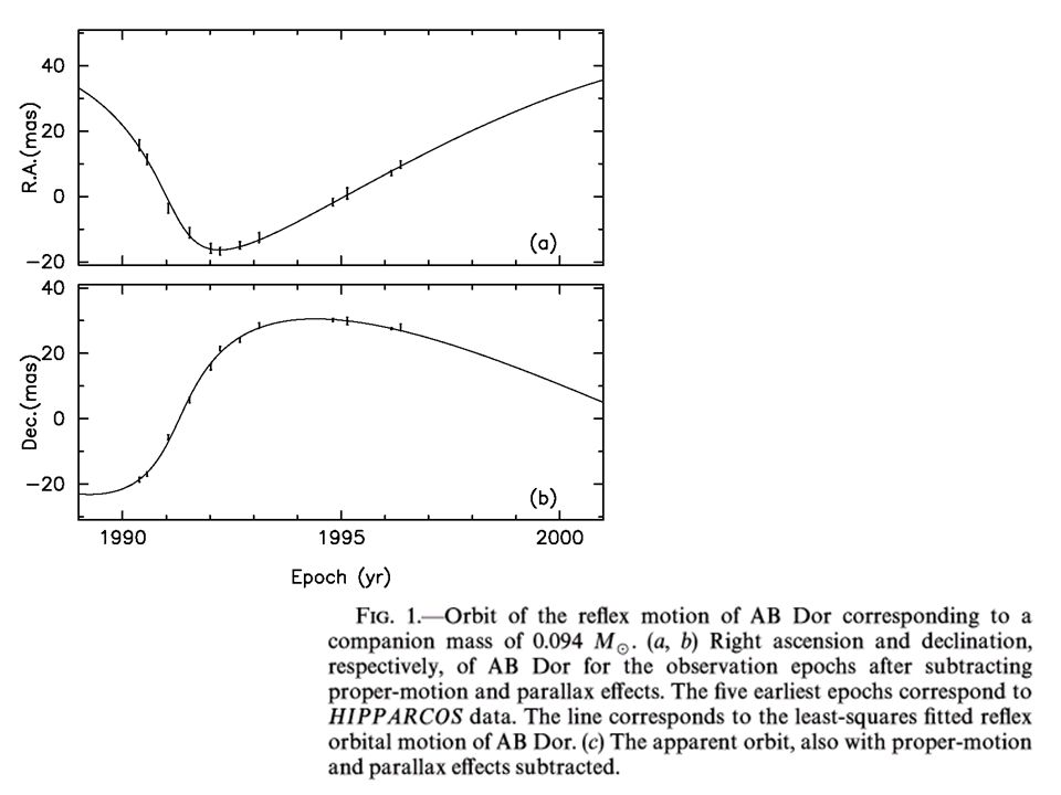
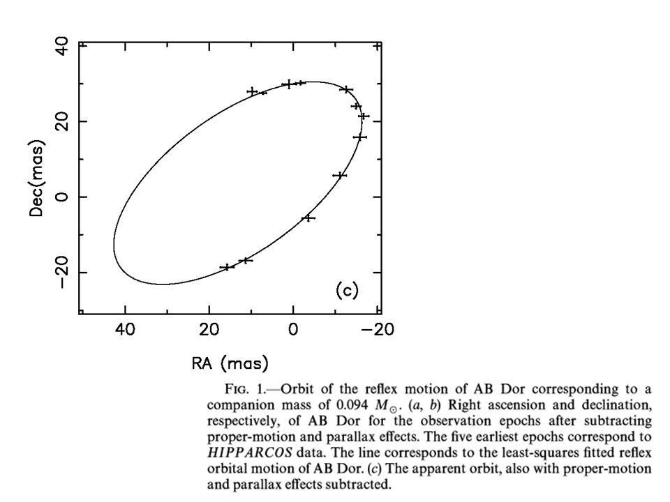
61. Exoplanet search