Download presentation
Presentation is loading. Please wait.

1
CHAPTER 3 Data Description

2
OUTLINE 3-1Introduction 3-2Measures of Central Tendency 3-3Measures of Variation 3-4Measures of Position 3-5Exploratory Data Analysis

3
OBJECTIVES Summarize data using the measures of central tendency, such as the mean, median, mode, and midrange. Describe data using the measures of variation, such as the range, variance, and standard deviation.

4
OBJECTIVES Identify the position of a data value in a data set using various measures of position, such as percentiles, deciles and quartiles. Use the techniques of exploratory data analysis, including stem and leaf plots, box plots, and five-number summaries to discover various aspects of data.

5
3-1 Introduction A statistic is a characteristic or measure obtained by using the data values from a sample. A parameter is a characteristic or measure obtained by using the data values from a specific population.

6
3-2 Measures of Central Tendency Mean Median Mode Mid-range

7
3-2 The mean (arithmetric average) meanThe mean is defined to be the sum of the data values divided by the total number of values.
 meanThe mean is defined to be the sum of the data values divided by the total number of values.")
8
3-2 The Sample Mean The symbol X represents the sample mean. X is read as “X - bar”. The Greek symbol Σ is read as “sigma” and means “to sum”.

9
The following data represent the annual chocolate sales (in millions of RM) for a sample of seven states in Malaysia. Find the mean. RM2.0, 4.9, 6.5, 2.1, 5.1, 3.2, 16.6

11
3-2 The Population Mean The Greek symbol µ represents the population mean. The symbol µ is read as “mu”. N is the size of the finite population.

12
A small company consists of the owner, the manager, the salesperson, and two technicians. Their salaries are listed as RM 50,000, 20,000, 12,000, 9,000 and 9,000 respectively. Assume this is the population, find the mean.

14
In a random sample of 7 ponds, the number of fishes were recorded as the following, find the mean. 23564536283337

15
3-2 The Sample Mean for an Ungrouped Frequency Distribution The mean for an ungrouped frequency distribution is given by f = frequency of the corresponding value X n = f

16
The scores of 25 students on a 4-point quiz are given in the table. Find the mean score. Score, XFrequency, f 02 14 212 34 43

17
Score, XFrequency, ff X 020 144 21224 3412 43

18
The number of balls in 17 bags were counted. Find the mean Number of ballsFrequency 55 64 72 86

19
3-2 The Sample Mean for a Grouped Frequency Distribution The mean for grouped frequency distribution is given by X m = class midpoint = (UCL + LCL) / 2
 / 2")
20
The lengths of 40 bean pods were showed in the table. Find the mean. Length (cm)Frequency, f 4-82 9-134 14-187 19-2314 24-288 29-335
Frequency, f")
21
Length (cm) Frequency, fMidpoint, X m f X m 4-82612 9-1341144 14-18716112 19-231421294 24-28826208 29-33531155
 Frequency, fMidpoint, X m f X m")
23
Time (in minutes) that needed by a group of students to complete a game are shown as below. Find the mean. Time (mins)Frequency 1-32 4-64 7-98 10-125 13-151
Frequency")
25
Mean = (fX) / n = 23 / 12 = 1.92 Mean = ( f X) / n = (12 x 10) / 12 = 10 Score, XFrequency, ffX 010 133 2510 326 414 X = 10n = f = 12 (f X) = 23
 / n = 23 / 12 = 1.92 Mean = ( f X) / n = (12 x 10) / 12 = 10 Score, XFrequency, ffX X = 10n = f = 12 (f X) = 23")
26
3-2 The Median When a data set is ordered, it is known as a data array. The median is defined to be the midpoint of the data array. The symbol used to denote the median is MD.

27
The ages of seven preschool children are 1, 3, 4, 2, 3, 5, and 1. Find the median. 1. Arrange the data in order. 2. Select the middle point.

29
In the previous example, there was an odd number of values in the data set. In this case it is easy to select the middle number in the data array. When there is an even number of values in the data set, the median is obtained by taking the average of the two middle numbers.

30
Six customers purchased these numbers of magazines: 1, 7, 3, 2, 3, 4. Find the median. 1. Arrange the data in order. 2. Select the middle point.

32
3-2 The Median - Ungrouped Frequency Distribution For an ungrouped frequency distribution, find the median by examining the cumulative frequencies to locate the middle value. If n is the sample size, compute n/2. Locate the data point where n/2 values fall below and n/2 values fall above.

33
LRJ Appliance recorded the number of VCRs sold per week over a one-year period. No. Sets SoldFrequency 14 29 36 42 53 Total24

34
To locate the middle point, divide n by 2; 24/2 = 12. Locate the point where 12 values would fall below and 12 values will fall above. Consider the cumulative distribution. The 12th and 13th values fall in class 2. Hence MD = 2.

35
This class contains the 5 th through the 13 th values. No. Sets SoldFrequencyCumulative Frequency 144 2913 3619 4221 5324 Median

36
3-2 The Median - Grouped Frequency Distribution For grouped frequency distribution, find the median by using the formula as shown below: Median, MD = L m + (W) n = sum of frequencies cf = cumulative frequency of the class immediately preceding the median class f = frequency of the median class w = class width of the median class L m = Lower class boundary of the median class
 n = sum of frequencies cf = cumulative frequency of the class immediately preceding the median class f = frequency of the median class w = class width of the median class L m = Lower class boundary of the median class")
37
Find the median by using the following data. ClassFrequency, f 16 - 203 21 - 255 26 - 304 31 - 353 36 - 402

38
ClassFrequency, fCumulative Frequency 16 - 2033 21 - 2558 26 - 30412 31 - 35315 36 - 40217

39
To locate the halfway point, divide n by 2; 17/2 = 8.5 ≈ 9. Find the class that contains the 9 th value. This will be the median class. Consider the cumulative distribution. The median class will then be 26-30.

40
=17 = = = –25.5=5 () ()= (17/2)–8 4 = 26.125. n cf f w L MD ncf f wL m m 8 4 30.5 25.5 2 525.5 ().
..")
41
Find the median by using the following data. ClassFrequency, f 5-145 15-247 25-3419 35-4417 45-547

42
3-2 The Mode The mode is defined to be the value that occurs most often in a data set. A data set can have more than one mode. A data set is said to have no mode if all values occur with equal frequency.

43
Find the mode for the number of children per family for 10 selected families. Data set: 2, 3, 5, 2, 2, 1, 6, 4, 7, 3. Ordered set: 1, 2, 2, 2, 3, 3, 4, 5, 6, 7. Mode: 2.

44
Six strains of bacteria were tested to see how long they could remain alive outside their normal environment. The time, in minutes, is given below. Find the mode. Data set: 2, 3, 5, 7, 8, 10. There is no mode since each data value occurs equally with a frequency of one.

45
Eleven different automobiles were tested at a speed of 15 mph for stopping distances. The distance, in feet, is given below. Find the mode. Data set: 15, 18, 18, 18, 20, 22, 24, 24, 24, 26, 26. There are two modes (bimodal). The values are 18 and 24.
. The values are 18 and 24..")
46
3-2 The Mode – Ungrouped Frequency Distribution ValuesFrequency, f 153 205 258 303 352 Mode Highest frequency

47
The mode for grouped data is the modal class. The modal class is the class with the largest frequency.

48
ValuesFrequency, f 15.5 - 20.53 20.5 - 25.55 25.5 - 30.57 30.5 - 35.53 35.5 - 40.52 Modal Class Highest frequency 3-2 The Mode – Grouped Frequency Distribution

49
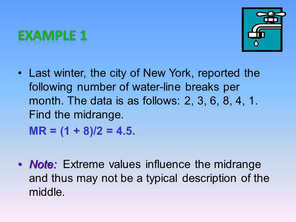
3-2 The Midrange The midrange is found by adding the lowest and highest values in the data set and dividing by 2. The midrange is a rough estimate of the middle value of the data. The symbol that is used to represent the midrange is MR.

52
3-2 Distribution Shapes Frequency distributions can assume many shapes. Three are three most important shapes: i) Positively skewed ii) Symmetrical iii) Negatively skewed
 Positively skewed ii) Symmetrical iii) Negatively skewed.")
53
Positively Skewed X Y Mode < Median < Mean Positively Skewed

54
Symmetrical n Y X Symmetrical Mean = Media = Mode

55
Negatively Skewed < Median < Mode

56
3-3 Measures of Variation Measure the variation and dispersion of the data. Range Variance Standard Deviation Coefficient of Variation

57
3-3 Range The range is defined to be the highest value minus the lowest value. The symbol R is used for the range. R = highest value – lowest value. Extremely large or extremely small data values can drastically affect the range.

58
3-3 Population Variance General Formula The symbol for population variance is. X = Individual value µ = Population mean N = Population size

59
3-3 Population Standard Deviation General Formula The population standard deviation is square root of the population variance.

61
ean = (10 + 60 + 50 + 30 + 40 + 20)/6 = 210/6 = 35.
/6 = 210/6 = 35.")
62
XX-µ(X-µ) 2 10-25625 60+25625 50+15225 30-525 40+525 20-15225 ∑X: 210 ∑(X-µ) 2 : 1750 The variance 2 = 1750/6 = 291.67. The standard deviation = 291.67 = 17.08

63
A class of 6 children sat a test; the resulting marks scored out of 10, were as follows: 456849 Calculate the mean, variance and standard deviation of this population.

64
3-3 Sample Variance General Formula The symbol for sample variance is. = Sample mean n = Sample size

65
3-3 Sample Standard Deviation General Formula The sample standard deviation is square root of the sample variance.

67
Mean, X = (35+45+30+35+40+25)/6 = 210/6 = 35
/6 = 210/6 = 35")
68
XX-X(X-X) 2 3500 45+10100 30-525 3500 40+525 -10100 ∑X: 210 ∑(X-X) 2 : 250 The variance 2 = 250/(6-1) = 50 The standard deviation = 50 = 7.07
 ∑X: 210 ∑(X-X) 2 : 250 The variance 2 = 250/(6-1) = 50 The standard deviation = 50 = 7.07")
69
Ungrouped frequency distribution Grouped frequency distribution How to find the population variance and standard deviation for data with frequency provided?

70
For ungrouped data, use the actual observed X value in the different classes. For grouped data, use the same formula with the X value replaced by class midpoints, X m.

71
Ungrouped frequency distribution Grouped frequency distribution How to find the sample variance and standard deviation for data with frequency provided?

72
Example XfXmXm fX m (X m - µ)(X m - µ) 2 f(X m - µ) 2 1-1045.522-10.59112.1481448.5924 11-20815.5124-0.590.34812.7848 21-30525.5127.59.4188.5481442.7405 N = 17 ∑fX m = 273.5 ∑f(Xm - µ) 2 = 894.1177
(X m - µ) 2 f(X m - µ) N = 17 ∑fX m = ∑f(Xm - µ) 2 =")
73
Mean, µ = ∑fX m / N = 273.5/17 = 16.09 Variance, 2 = 894.1177 / 17 = 52.60 Standard deviation, = 2 = 52.60 = 7.25

74
Question a) The scores in a statistics test for 60 candidates are shown in the table. Find the mean, variance, and standard deviation for this population. ScoreFrequency 0-198 20-3913 40-5924 60-7911 80-994

75
b) The following table showed the number of cars passed by UM hospital in a random sample of days. Compute the sample mean, variance and standard deviation. Number of carsNumber of days 101-1202 121-1304 131-14015 141-15010 151-1607

76
3-3 Coefficient of Variation The coefficient of variation is defined to be the standard deviation divided by the mean. The result is expressed as a percentage. It is used to compare the standard deviation of different units. CVar s X orCVar 100%100%. =

78
3-3 Chebyshev’s Theorem 75% of the values will lie within 2 standard deviations of the mean. Approximately 89% will lie within 3 standard deviations.

80
3-3 Empirical (Normal) Rule For any bell shaped distribution: Approximately 68% of the data values will fall within one standard deviation of the mean. Approximately 95% will fall within two standard deviations of the mean. Approximately 99.7% will fall within three standard deviations of the mean.

81
-- 95%

82
Question The scores on a national achievement exam have a mean of 480 and standard deviation of 90. If the scores are normally distributed, find the scores for approximately 68% of the data values, 95% of the data values, and 99.7% of the data values.

83
3-4 Measures of Position Measure the position of particular data in a data set. Z - score Percentile Decile Quartile

84
3-4 Z-Score The standard score or z score for a value is obtained by subtracting the mean from the value and dividing the result by the standard deviation. The symbol z is used for the z score. Z = (value - mean)/ standard deviation
/ standard deviation.")
85
The z score represents the number of standard deviations a data value falls above or below the mean. Forsamples z XX s Forpopulations z X :. :.

86
A student scored 65 on a statistics exam that had a mean of 50 and a standard deviation of 10. Compute the z-score. z = (65 – 50)/10 = 1.5. That is, the score of 65 is 1.5 standard deviations above the mean. Above - since the z-score is positive. How about if the z-score shows a negative value?
/10 = 1.5. That is, the score of 65 is 1.5 standard deviations above the mean. Above - since the z-score is positive. How about if the z-score shows a negative value .")
87
3-4 Percentile Percentiles divide the distribution into 100 equal groups. P 1 P 2 P 3 P 4 ……………… P 98 P 99 P 100

88
How to find the Value Corresponding to a Given Percentile? Step 1: Arrange the data in order. Step 2: Compute c = (n p)/100. c = position value of the required percentile p = percentile n = sample size
/100. c = position value of the required percentile p = percentile n = sample size.")
89
Step 3: If c is not a whole number, round up to the next whole number and find the corresponding value. If c is a whole number, use the value halfway between c and c+1.

90
Find the value of the 25th percentile for the following data set: 18, 12, 3, 5, 15, 8, 10, 2, 6, 20.

91
Is the data arranged in order? Arrange data in order form: 2, 3, 5, 6, 8, 10, 12, 15, 18, 20. n = 10, p = 25, so c = (10 25)/100 = 2.5. Since 2.5 is not a whole number, round up to c = 3. Thus, the value of the 25th percentile is the value X = 5.
/100 = 2.5. Since 2.5 is not a whole number, round up to c = 3. Thus, the value of the 25th percentile is the value X = 5..")
92
3-4 Decile Deciles divide the data set into 10 groups. D 1 D 2 D 3 D 4 D 5 D 6 D 7 D 8 D 9 D 10

93
What is the relationship between percentile and decile? D 1 corresponding to P 10 D 2 corresponding to P 20 D 9 corresponding to P 90 D 10 corresponding to P 100

94
3-4 Quartile Quartiles divide the data set into 4 groups. Q 1 Q 2 Q 3 Q 4

95
What is the relationship between percentile and quartile? Q 1 corresponding to P 25 Q 2 corresponding to P 50 Q 3 corresponding to P 75 Q 4 corresponding to P 100 Median

96
3-4 Outliers and the Interquartile Range (IQR) An outlier is an extremely high or an extremely low data value when compared with the rest of the data values. The Interquartile Range, IQR = Q 3 – Q 1.

97
Procedures to identify outliers To determine whether a data value can be considered as an outlier: Step 1: Arrange the data in order. Step 2: Compute Q 1 and Q 3. Step 3: Find the IQR = Q 3 – Q 1. Step 4: Compute (1.5)(IQR).
(IQR)..")
98
Step 5: Compute Q 1 – (1.5)(IQR) and Q 3 + (1.5)(IQR). Step 6: Compare the data value (say X) with Q 1 – (1.5)(IQR) and Q 3 + (1.5)(IQR). If X Q 3 + (1.5)(IQR), then X is considered an outlier.
 with Q 1 – (1.5)(IQR) and Q 3 + (1.5)(IQR). If X Q 3 + (1.5)(IQR), then X is considered an outlier..")
100
Find Q 1. Q 1 is corresponding to P 25 c = (np)/100 = (825)/100 = 2 nd Since 2 is a whole number, take value between 2 nd and 3 rd. Q 1 = (6+12)/2 = 9
/100 = (825)/100 = 2 nd Since 2 is a whole number, take value between 2 nd and 3 rd. Q 1 = (6+12)/2 = 9.")
101
Find Q 3. Q 3 is corresponding to P 75 c = (np)/100 = (875)/100 = 6 th Since 6 is a whole number, take value between 6 th and 7 th. Q 3 = (18+22)/2 = 20
/100 = (875)/100 = 6 th Since 6 is a whole number, take value between 6 th and 7 th. Q 3 = (18+22)/2 = 20.")
102
Find IQR. IQR = 20 - 9 = 11. (1.5)(IQR) = (1.5)(11) = 16.5. 9 – 16.5 = – 7.5 and 20 + 16.5 = 36.5. The value of 50 is outside the range – 7.5 to 36.5, hence 50 is an outlier.

103
3-5 Exploratory Data Analysis - Stem and Leaf Plot A stem and leaf plot is a data plot that uses part of a data value as the stem and part of the data value as the leaf to form groups or classes. Leaf Stem

104
Example of Stem and Leaf Plot 42 5 2 5 Stem Leaves

105
Stem Leading digit Leaf Trailing digit

106
At an outpatient testing center, a sample of 20 days showed the following number of cardiograms done each day: 25, 31, 20, 32, 13, 14, 43, 02, 57, 23, 36, 32, 33, 32, 44, 32, 52, 44, 51, 45. Construct a stem and leaf plot for the data.

107
Leading Digit (Stem) Trailing Digit (Leaf) 012345012345 2 3 4 0 3 5 1 2 2 2 2 3 6 3 4 4 5 1 2 7
 Trailing Digit (Leaf)")
108
3-5 Exploratory Data Analysis - Box Plot When the data set contains a small number of values, a box plot is used to graphically represent the data set. These plots involve five values: 1. Minimum value 2. Q 1 3. Median 4. Q 3 5. Maximum value

109
Example of Box Plot Minimum valueMaximum value Q2Q2 Q1Q1 Q3Q3

110
Information Obtained from a Box Plot If the median is near the center of the box, the distribution is approximately symmetric. If the median falls to the left of the center of the box, the distribution is positively skewed. If the median falls to the right of the center of the box, the distribution is negatively skewed.

111
If the lines are about the same length, the distribution is approximately symmetric. If the right line is larger than the left line, the distribution is positively skewed. If the left line is larger than the right line, the distribution is negatively skewed.

Similar presentations


 MSIS 111 Prof. Nick Dedeke.>")


2000 South-Western College Publishing.>")


>")
