1. Describing and Displaying Quantitative data

2. Summarizing continuous data Displaying continuous data Within-subject variability Presentation

3. Summarizing continuous data A quantitative measurement contains more information than categorical. The two most important pieces of information about quantitative measurement are Where is it ? How variable is it? These are the central tendency and measure of spread (variability)

4. Measure of central tendency

5. Example students record student\subjectsubj1subj2subj3subj4Mean s12878187 s233625850 s33989967 s436588029 s537988178 s61973872 s788119258 s880411342 s940114811 s1097931847

6. students record student\subjectsubj1subj2subj3subj4Mean s1287818751 s23362585051 s33989967 s43658802951 s53798817874 s6197387252 s78811925862 s88041134244 s94011481128 s109793184764

7. Mean or average is a statistical sense and efficient. Outliers are single observations which have noticeable influence on the results. These outliers should be excluded from the sample. Outliers should be excluded from the final data summary.

8. BabyWeight (kg) B11.2 B21.3 B31.4 B41.5 B52.1 Mean1.5

9. BabyWeight (kg) B11.2 B21.3 B31.4 B41.5 B521 Mean7.89

10. Medianis estimated by first ordering the data from smallest to largest, and then counting upwards for half of the observations, the center observation in odd samples or the average of middle two observations in even samples.

11. Example students record student\subjectsubj1subj2subj3subj4MeanMedian s128781875154.5 s2336258505154 s33989967 82.5 s4365880295147 s5379881787479.5 s6109738725455 s7881192586273 s8804113424441.5 s9401148112825.5 s10100 98859699 s11979318476470 average50.261.4564.1856.9158.1818 Median3762805854.25

12. Median measure it will not be affected by the outliers.

13. Mode More is the value that occurs most frequently, if the data grouped then it will be the grouping with highest frequency. It is useful for categorical data to report the most frequent category.

14. Example

15. Measures of Dispersion or variability Range and interquartile range Range is the smallest and largest observations, to measure the variability. Example : In age variable we would like to know the youngest and oldest participant. Outliers presence will give distorted impression about the variability

16. Quartiles namely are lower, median and upper quartile, which divide the data into four equal parts. First order the data and then count the appropriate number from bottom. the interquartile range is useful measure of variability and is given by the difference of lower and upper quartiles.

17. Example Meanquartiles 28 44 51 lower quartiles (25th percentile)51 median quartile (50th percentile)53 54 62 67 upper quartile (75th percentile)67 74 96 interquartile rangefrom 51 to 67

18. Interquartile is not vulnerable to outliers. Here we know that 50% of the data lie within the interquartile range

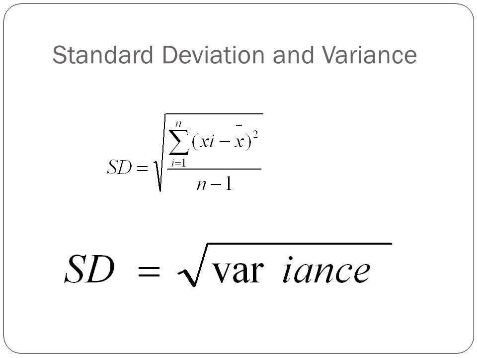
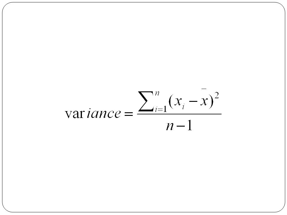
19. Standard Deviation and Variance

22. Example students record student\subjectsubj1subj2subj3subj4Standard Deviation s1287818739.4 s23362585012.8 s3398996745.0 s43658802923.1 s53798817825.9 s61097387238.1 s78811925837.4 s88041134227.5 s94011481119.3 s10100 98857.2 total standard deviation 31.7

23. Why Standard deviation is useful? Dark blue is less than one standard deviation from the mean. For the normal distribution, this accounts for 68.27 % of the set; while two standard deviations from the mean (medium and dark blue) account for 95.45%; three standard deviations (light, medium, and dark blue) account for 99.73%; and four standard deviations account for 99.994%.normal distribution

24. Example : The median age of menopause for cases as 50.1 years and the interquartile range is 48.6 to 52.5, thus we know that 50% of the women experienced the menopause within 4-years age range

25. Displaying Continuous Data A picture worth thousand words, or numbers, so there is no better way to present the data than figures of graph The graph or figure should convey as much information as possible. With one constraint that the reader is not overwhelmed by too much data

26. Dot plot Example

27. Histogram : used with huge numerical data, where the data will be divided none overlapping intervals, then counting the number of observations in each. example

28. Box whisker plot more compact information can be visualized The whiskers in the diagram indicate the minimum and maximum values of the variable under consideration. The median value is indicated by the central horizontal line. The lower and upper quartile by the corresponding horizontal ends of the box. The shaded box itself represents the interquartile range.

29. The box-whisker plot is used to display median and two measure of spread, namely the range and interquartile.

30. Scatter plot It used to illustrate the relationship between two continuous variables

31. Measures of Symmetry Dot and histogram plots give us idea about the shape of the distribution of the data. Symmetric: means if you fold the shape over the central point the two halves will agree other wise will call it skewed, either left skewed or right skewed. If the distribution is symmetric then the mean and the median will be close to each other.

32. If the distribution is skewed then the median and interquartile range are the approperiate summary measure than mean and standard deviation. Standard deviation and mean are sesitive to the skewness. Example : If we have mean = 1.31 and median = 1.34 we can conclude that the data are reasonably symmetric

33. Example: If we have the median = 50.1 but it is not exactly in the mid of the first and third quartile of 48.6 and 52.5 which indicate the skewness in the data distribution.

34. Within the subject variable Measurement taken once for the subject (weight of the baby) and the variability expressed by standard deviation we call it between-subject variability ( the subject not changing frequently) Measurements taken repeatedly on one subject then we are assessing within-subject variability. ( the subject changing frequently)

35. Within-subject values are unlikely to be independent. Consecutive values will be dependent on values proceeding them In the investigation of total variability it is very important to distinguish within-subject from between-subject variability. The experimenter must be aware of possible sources which contribute to the variation, decide which are of importance in the intended study, and design the study appropriately.

36. Exercise The age (in years) of a sample of 20 motor cyclists killed in road traffic accidents is given below: Calculate the mean, median, and mode. Calculate the range, inter quartile range and standard deviation. Which of these is better to describe the variability of these data? Draw a dot plot and histogram. Is this distribution symmetric or skewed? 18412428715215202131 16243344202416642432

37. Mean= 30.9 Median= 24 Mode= 24 SD =15.93705

38. Age classesFrequency 10-151 15-3314 33-523 More2

39. Min15 Max71 Range56 Quarter 120 Quarter 335 Interquartile15