1. Digital Image Processing DIGITIZATION

2. Summery of previous lecture Digital image processing techniques Application areas of the digital image processing History of image processing techniques Steps in digitization of images

3. Todays lecture Why do we need to digitization? What is digitization? How to digitize an image?

4. Why digitization we need?

5. Theory of real numbers: between any two given points there are infinite numbers of points. An image is represented by infinite number of points Its not possible to represent infinite number in computer

6. Digitization 1: An image shall be represented in a form of a finite 2D matrix 2: The element values of f should also be finite

7. Image as a matrix of numbers representation

8. What is digitization ? Image representation by D2 finite matrix (sampling) Values of the Elements at the matrix are from the finite set of discrete values (quantization)

9. To process images we need To digitize the image – Sampling (we will focus on it) – Quantization – To visualize the image it needs to for displaying the images, it has to be first converted into the analog signal which is then displayed on a normal display.

10. Sampling, Quantization and display

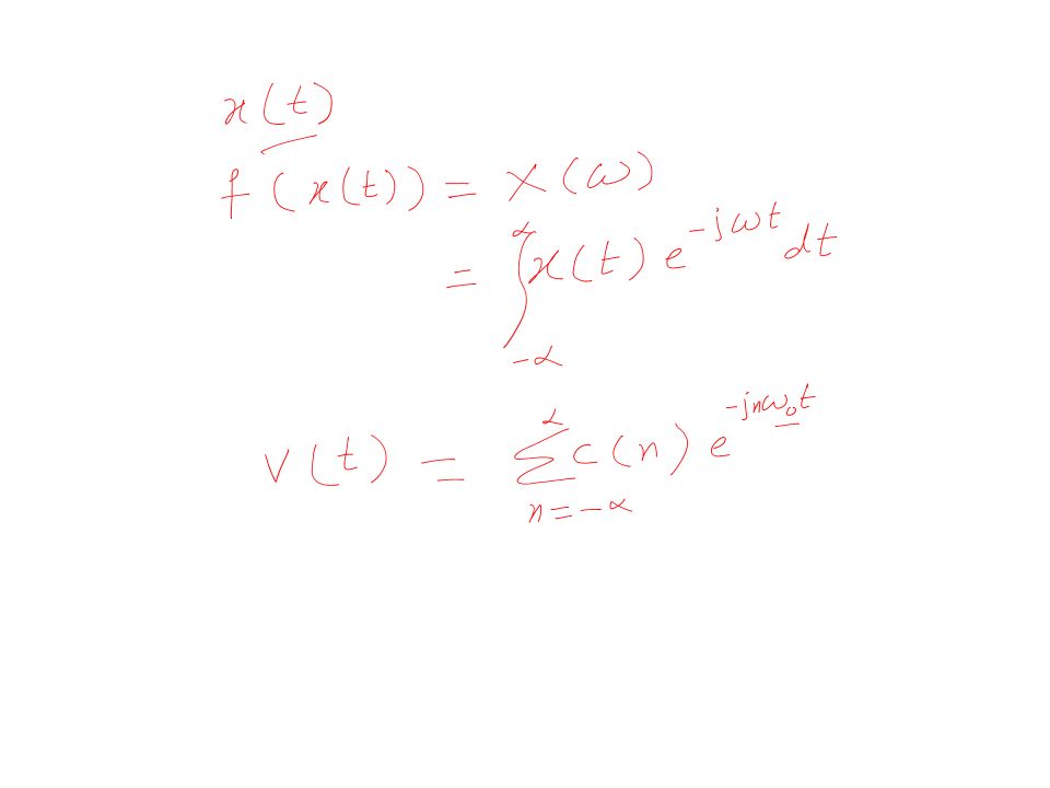
11. Sampling 1 D sampling Assuming that we have a 1 dimensional signal x (t) Which is a function of t. Here, we assume this t to be time It is known that whenever some signal is represented as a function of time; signal is represented in the form of hertz Hertz means it is cycles per unit time.

12. Sampling Instead of taking considering the signal values at every possible value of t; consider the signal values at certain discrete values of t. X (t) at t equal to 0. the signal X (t) at t equal to 2 delta t S The value of signal X (t) at t equal to delta 2 t S, at t equal to delta 3 t S and so on. delta t S is the sampling interval and corresponding sampling frequency is represent it by f S, it becomes 1 upon delta t S. Issue is local minimum, local maximum,

13. Sampling issue increase the sampling frequency or decrease the sampling interval. make the new sampling interval represented as delta t S dash which is equal to delta t S by 2. The sampling frequency is f S dash equal to 1 upon delta t S dash, twice of f S. The earlier sampling frequency of f S, and now its delta 2 f S, twice f S

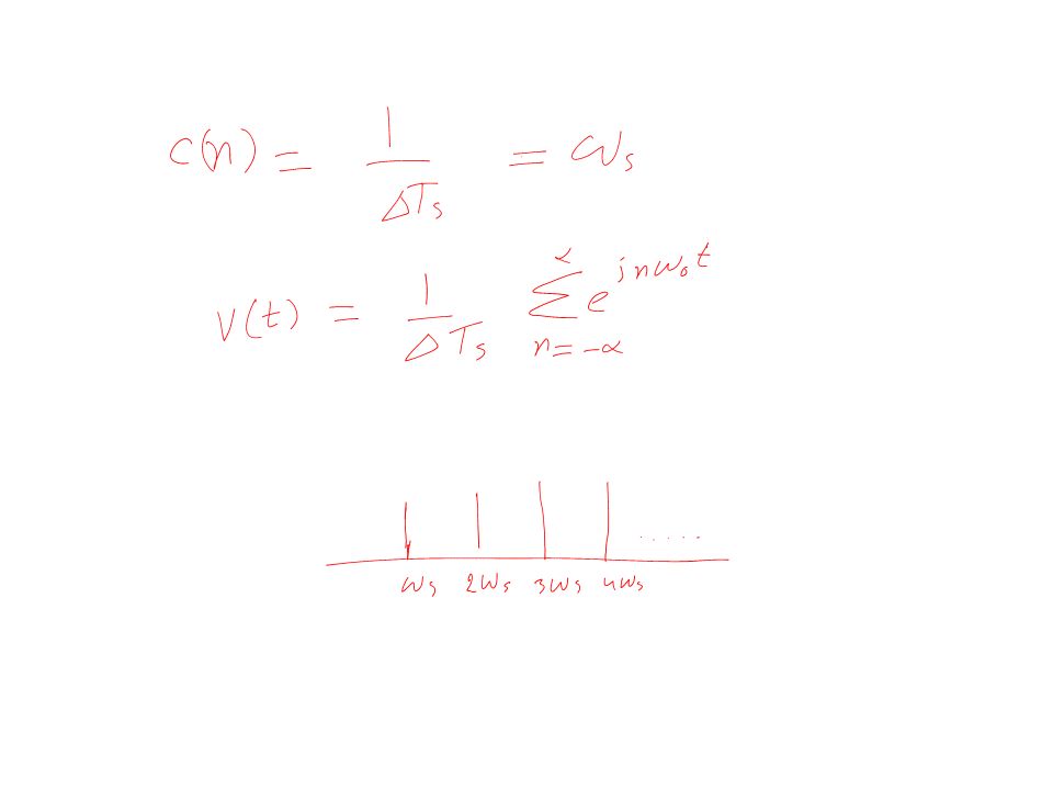
14. Theory of sampling Each of these are sequences of Dirac delta functions and the spacing between 2 delta functions is delta t. In short, these kind of function is represented by comb function, a comb function t at an interval of delta t and delta t minus m into delta t, where m varies from minus infinity to infinity.

15. Dirac delta function Dirac delta function delta t, the functional value will be 1 whenever t equal to 0 the functional value will be 0 for all other values of t. In this case, when delta t minus m of delta t, this functional value will be 1 only when this quantity that is (t minus m delta t) becomes equal to 0. That means this functional value will assume a value 1 whenever t is equal to m times delta t for different values of m varying from minus infinity to infinity.

16. Theory of sampling These samples can now be represented by multiplication of X (t) with the series of Dirac delta functions that we have seen that is comb of t delta t. So by multiply, whenever this comb function gives a value 1; only the corresponding value of t will be retained in the product and whenever this comb function gives you a value 0, the corresponding points, the corresponding values of X (t) will be said to 0.

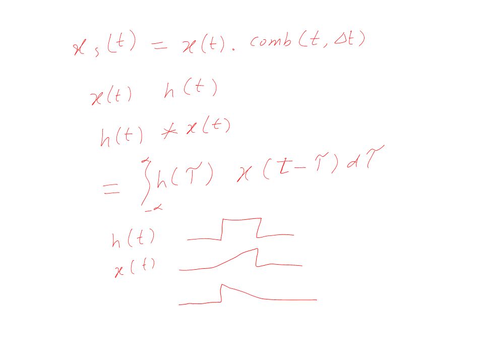
17. The discretization process can be represented mathematically as x S (t) is equal to X (t) into comb of t delta t and If expand the comb function and consider only the values of t where this comb function has a value 1, then this mathematical expression is translated to x of m delta t into delta t minus m delta t where m varies from minus infinity to infinity.

18. Sampling from signal The sampling will be proper if its to be reconstruct the original continuous signal X (t) from these sampled values For that needs to maintain certain conditions so that the reconstruction of the analog signal X (t) is possible.

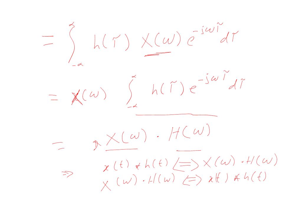
27. Reconstruction In time domaine One signal is X (t), the other signal is comb function, comb of t delta t. So, these relations, as these are true that if multiply 2 signals X (t) and y (t) in time domain that is equivalents to convolution of the 2 signals x omega and y omega in the frequency domain. For Sampling we have got x s (t) that is the sampled values of the signal X (t) which is nothing but multiplication of X (t) with the series of Dirac delta functions represented by comb of t delta t. it is equivalent to in frequency domain, x S of omega which is equivalent to the frequency domain representation x omega of the signal X (t) convoluted with the frequency domain representation of the comb function, comb t delta t and the comb function is the Fourier transform or the Fourier series expansion of this comb function which is again a comb function.

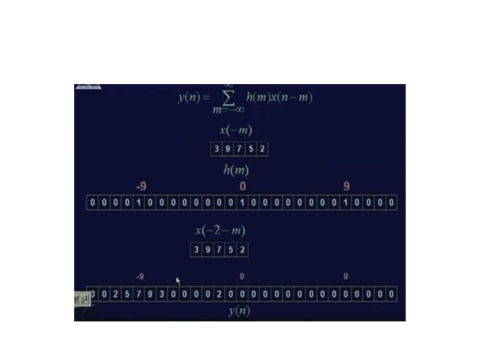
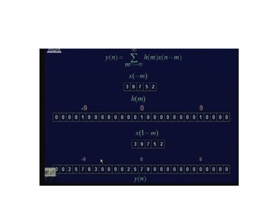
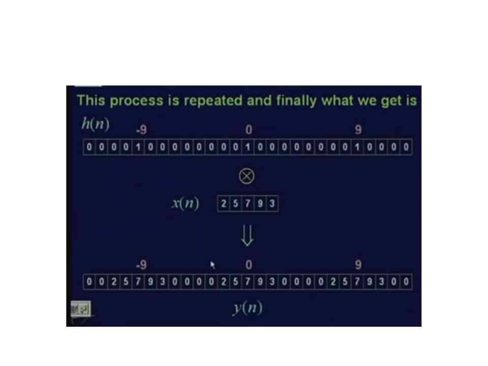
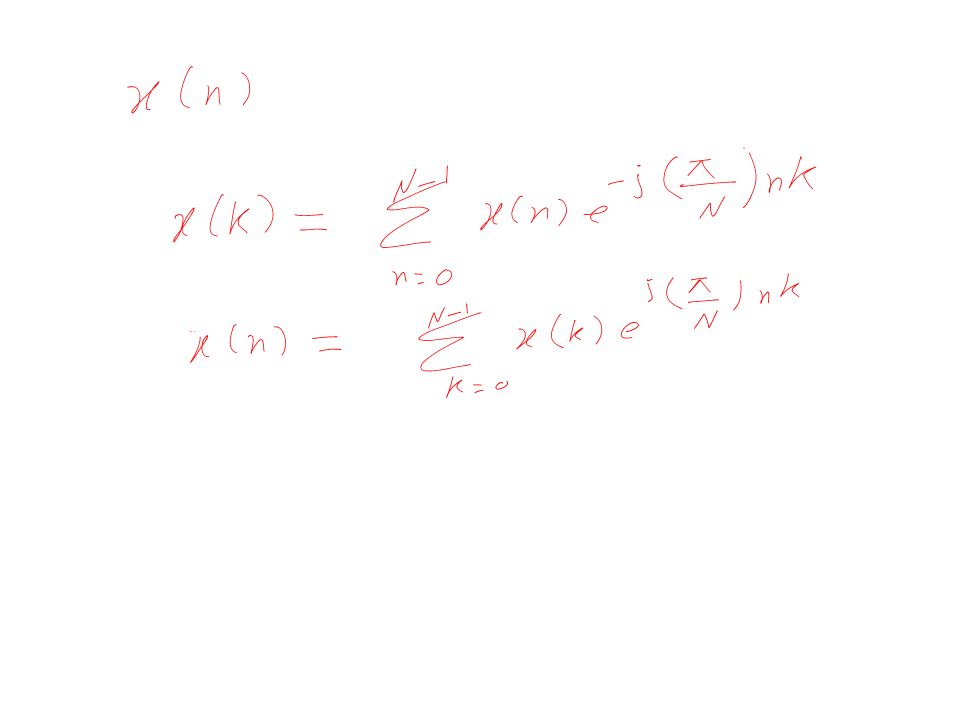
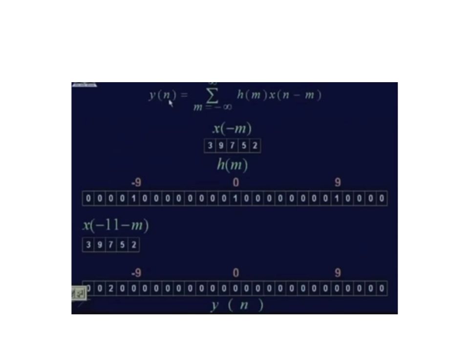
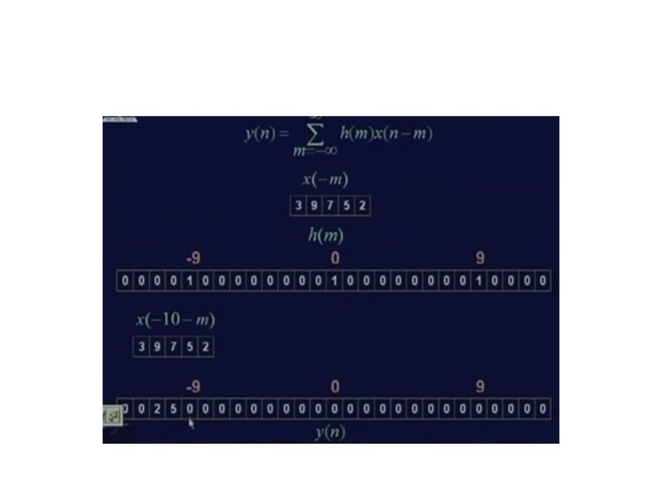
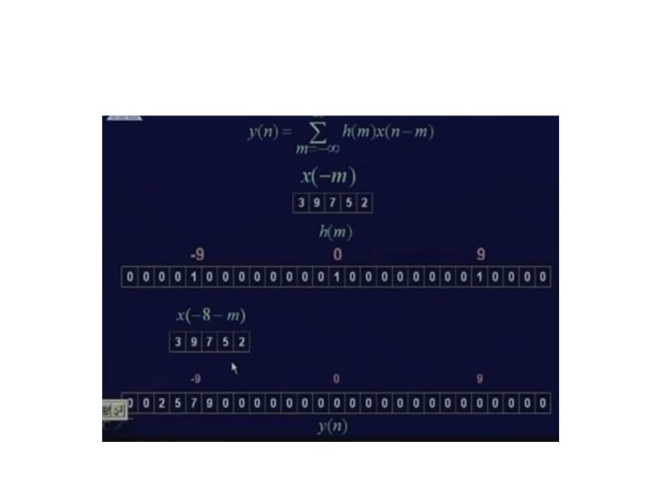
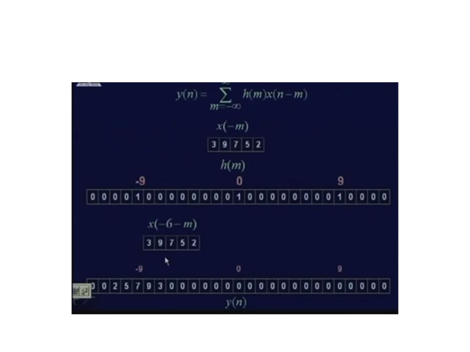
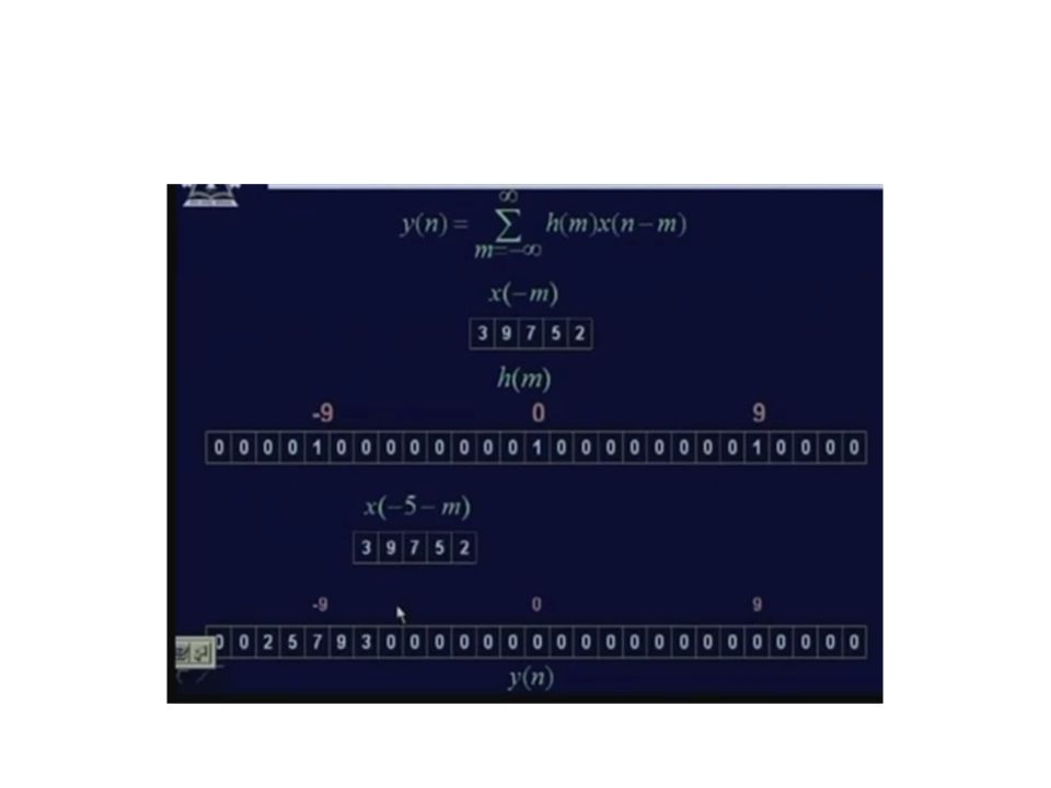
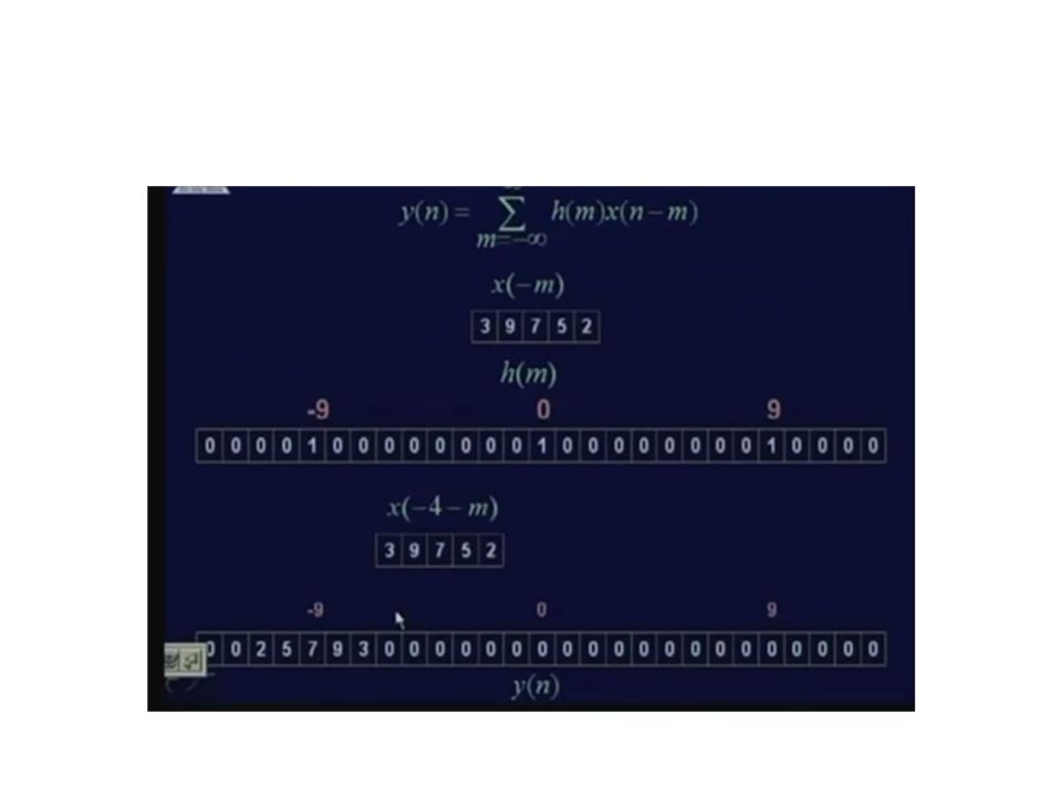
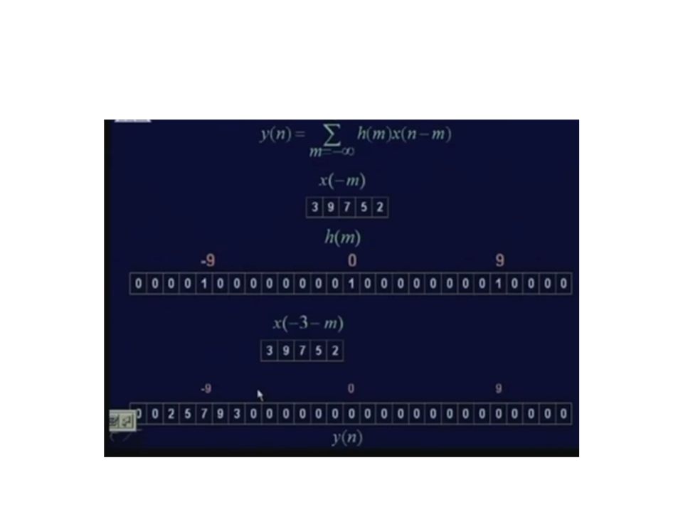
28. Convolution 2 signals h (n) and x (n) are in the sample domain. h (n) is nothing but a comb function where the delta t S have value of h (n) is equal to 1 at n equal to 0, … In discrete data domain, the convolution expression is translated to y (n) equal.. So, let us see that how this convolution actually takes place.

43. Convolute 2 signals X (t) and the Fourier transform of this comb function that is comb omega in the frequency domain

44. When X (t) is band limited, that means the maximum frequency component in the signal X (t) is omega naught; then the frequency spectrum of the signal X (t) which is represented by x omega With low pass filter whose cut off frequency is just beyond omega naught and this frequency signal, will pass through low pass filter and will just take out this particular frequency band and it will cut out all other frequency bands.

45. The frequency gap between this frequency band and this translated frequency band are The difference of between center of frequency band and the other center of frequency band is nothing but 1 upon t S which is equal to omega s that is the sampling frequency. As long as this condition that is 1 upon t S minus omega naught is greater than omega naught, that is the lowest frequency of this translated frequency band is greater than the highest frequency of the original frequency band; then only these 2 frequency bands are disjoint and when these 2 frequency bands are disjoint, then only by use of a low pass filter, I can take out this original frequency band.

46. References Prof.P. K. Biswas Department of Electronics and Electrical Communication Engineering Indian Institute of Technology, Kharagpur Gonzalez R. C. & Woods R.E. (2008). Digital Image Processing. Prentice Hall. Forsyth, D. A. & Ponce, J. (2011).Computer Vision: A Modern Approach. Pearson Education.