1. Totally constrained systems with discrete evolution parameter Rodolfo Gambini In collaboration with Jorge Pullin

2. During the last years we have developed a canonical procedure for the treatment of discrete constrained systems. Even if one considers that the final theory should be continuous, which is not obvious, discretizations play a crucial role at the intermediate steps. In fact they are required for numerical computations and provide a regularization for quantum field theory and probably for quantum gravity. Discretizations present considerable difficulties: In Numerical Relativity the constraints are not preserved by the discrete evolution and the description is inconsistent. At the quantum level, Regge calculus and the spin foam formalism lead to problems related with the integration measure and the recovery of the continuum limit. Finally in Loop Quantum Gravity some of the ambiguities of the dynamics may be traced back to the discrete theory.

3. When this approach, usually called consistent discretizations, is applied to G.R., one does not fix a gauge but nevertheless the theory is constraint free. This allows to solve many of the hard conceptual problems of general relativity. At the classical level it preserves the constraints with a high degree of approximation and at the quantum level the theory has the same kinematics than loop quantum gravity. Discrete Canonical formalism.

4. Relations that define a type 1 canonical transformation

5. Canonical formulation for constrained discrete dynamical systems

6. The final evolution equations are obtained by substituting the Lagrange multipliers. Notice that here the Lagrange multipliers were determined without imposing any gauge fixing. Notice that more precisely what has been determined is For a completely parameterized theory there is no explicit dependence on epsilon, which may be fixed arbitrarily. Once the time interval (or the lattice spacing) is chosen, the lapse is determined. When And one recovers the continuum limit.

7. “Dirac’s” canonical approach to general discrete systems. = 0 Primary constraints V and U arbitrary functions Consistency:

8. By using a Type II, III, or IV transformation one can show that this evolution is canonical, preserves the Poisson brackets and the constraint surface. This is equivalent to what happens in the continuum, where consistency may be achieved by determining the complete constraint surface and a total Hamiltonian that preserves the Poisson structure Finally one can recognize the second class constraints and impose them strongly. While some symmetries of the continuum are broken by the discretization others are preserved.

9. Class.Quant.Grav.19:5275-5296,2002 C.Di Bartolo, R. Gambini and J.Pullin The procedure has been extended to quantum field theories and reproduces, for usual gauge theories as Yang-Mills, the standard results obtained by using transfer matrix techniques on a lattice. The procedure also provides a very simple description of B-F theories on a lattice. General relativity may be discretized in several ways. One can start from the standard ADM formalism or use Ashtekar’s variables. I will discuss later on the use of Regge Calculus.

10. . In the case of general relativity the gauge invariance and the invariance under spatial diffeomorphisms may be exactly preserved and the final quantum theory may be in principle treated in terms of loops making use of the Ashtekar Lewandowski measure. At the classical level, the procedure is computationally intensive in a generic situation, requiring the simultaneous solution of ten coupled non linear equations at each lattice point. We have recently completed the classical study of the Gowdy models and shown that the constraints are preserved with a good degree of precision during evolution. R.G and J. Pullin Phys. Rev. Lett. 90 021301 2003 R.G. M. Ponce and J. Pullin Phys Rev. D 72 024031 2005

11. 4 Issues 1)Existence of global descriptions: Is it possible to cover the complete classical orbits? 2) Canonical description for geometric actions of G.R. like the Regge action within the consistent discretization approach. 3) The Issue of time and a description of the evolution in terms of conditional probabilities. 4) Unitary implementation of classical canonical transformations.

12. An example of a totally constrained system without a global time variable.

13. An example of application: The Regge Action. The continuum Regge action in D=2 and D=3. In 2 dimensions: (n,m) In two dimensions the classical action is not determined by the initial and final one dimensional complex that does not have any information about the intrinsic curvature, and it needs to be modified. One usually considers the discrete version of the Polyakov string which has additional information about the embedding of the lattice. In this case, besides the Regge length variables we need the coordinates of the points in the target space

14. For reasons of simplicity I discuss here the 2 dimensional case. The analysis of the 3D system follows similar lines. play the role of Lagrange multipliers and are fixed in terms of the canonical pair by the previous eqs. They also determine the evolution equation: And finally from the definition of the canonical momentum at level n+1 we get The remaining evolution equation.

15. Each prism is decomposed in three tetrahedra: (1)In ABA’D, DEE’D, DEAA’ (2) In ABB’D, AB’D’D, A’FDD’ The quantization of the system determines the Euclidean or unitary evolution operator.

16. The consistent discretization scheme uniquely determines the integration measure in the Path Integral. This measure differs from the standard measures usually considered in Regge calculus: While here: We haven’t checked yet if the resulting transition amplitudes present the same pathologies than the standard Regge amplitudes.

17. A solution to the problem of time. Standard quantum mechanics presupposes the existence of an externally defined classical variable called t. The other variables, x play a very different role and are represented by operators. This is clearly an approximation that requires the existence of a classical clock external to the system, and will not be very useful in the context of closed systems where everything behaves quantum mechanically, as the Universe close to the Big Bang. Page and Wooters proposed to treat all variables quantum mechanically and use one of them as a clock as long as it behaves semi-classically. However, in standard canonical quantum gravity and other totally constrained systems the idea runs into problems. The clock variable must change during evolution, and therefore it cannot commute with the constraints. This implies that it will not be well defined on the physical space of states annihilated by the constraints. If one tries to work in the kinematical space, the wave functions corresponding to physical states are distributional and cannot be used to construct a probabilistic interpretation.

18. Thus, up to present, the description of the time evolution in totally constrained systems has always involved a classical clock variable. Either by fixing a gauge or by introducing Rovelli’s evolving constants. Relational Time. The elimination of the constraints associated with the reparameterizaton Invariance simplify all the quantization process and allows to treat in a simpler way old conceptual problems as the issue of time. Notice that the evolution variable n does not have any intrinsic meaning and it is not associated with any dynamical variable. We shall introduce time via conditional probabilities. In many simple models with discrete evolution, the physical and the kinematical spaces coincide. For instance in a cosmological model with two degrees of freedom A, Φ:

19. Loss of coherence. It will be convenient to introduce conditional probabilities for a state given in terms of a density operator. Let us now assume that the clock and the system are weakly interacting in such a way that:

20. and assume the existence of a semi-classical regime for the variable chosen as time in a given initial state of the clock. That means that n and time are strongly correlated. is the probability that the measurement t corresponds to the value n.

21. Now, one can define a time dependent density operator Such that the conditional probability takes the usual form We have therefore ended with the standard probability expression with an effective density matrix in the Schroedinger picture. It is evident from its definition that exact unitarity is lost, since we end up with a statistical mixture of states associated with different n’s. This fact leads to a modification of the Schroedinger equation for any quantum system whose evolution is described with real clocks. I will not analyze here the physical consequences of this result. R.G., R. Porto, J.Pullin: NJP6,45(2004)

22. Quantum unitary implementations of the canonical transformations. The relational procedure that we have introduced here allowed us to describe the evolution in terms of conditional probabilities defined in terms of a quantum clock variable. However, as it is well known, and was extensively discussed by Arlen Anderson many canonical transformations do not lead to unitary transformations or isometric transformations at the quantum level. This is the case when one trays to recover the standard quantum mechanics starting from a totally constrained system with a quantum relational time. We shall see that for this kind of systems the implementation of the canonical transformations at the quantum level by unitary transformations requires restricting the kinematical Hilbert space.

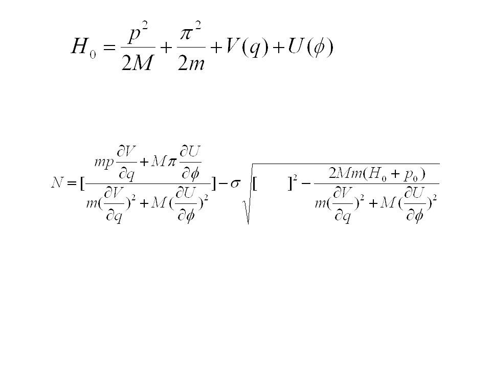
23. Substituting the Lagrange multiplier N in the evolution equations one gets the canonical transformations connecting level n and n+1 The step of the evolution is governed by C a quantity that vanishes in the continuum limit.

25. The 4 independent perennials of the continuum theory are constants of the motion of the discrete counterpart. The choice of the sign σ is made to insure that the sign of Δ is preserved by the evolution. At the turning point of the macroscopic particle one needs to change the branch of the lapse.

26. Quantization: How to find a unitary implementation of the evolution. We start by choosing a polarization. In order to simplify the determination of the evolution operator we choose to work in a kinematical space with square integrable wave-functions such that: The classical evolution given by canonical transformations needs to be implemented at the quantum level by unitary operators.

27. And as usual U can be interpreted as the transition amplitudes between eigenstates of the operators in the Heisenberg picture at levels n and n+1. To determine U one needs to impose the evolution equations. For instance: And similarly for the other variables. Solving these equations one gets U. However, U is unitary only in the space expanded by the negative eigenvalues of With Δ<0 Notice that here is a subspace of the kinematical space!

28. By construction the evolution preserves As usual only the observables such that are well defined in the physical space. But now, not only the constants of the motion are observable, the operator associated to the position of the macroscopic variable is also observable because. This fact is basic for a relational description of the evolution. Relational time and continuum behavior. One can recover the standard quantum mechanical description using q as the clock variable and working in the continuum regime where;

29. The quantum continuum regime is reached by considering states such that: 1)The mean value of the operator that measure the step of the evolution is small. 2) The evolution preserves the continuum regime. 3) The measurement of any admissible dynamical variable preserves this regime. We have shown that these conditions are compatible and one can define a time dependent density operator such that: Where ρ satisfies the standard Schroedinger equation plus corrections.

30. CONCLUSIONS In the last year we have made several advances within the consistent discretizations approach. We now know how to approach the complete continuum orbit y a totally constrained system. We have shown that the Regge action may be treated within this approach leading to a non trivial constraint structure. This seems to be the most natural way of treating general relativity in a discretized scheme. We have made progress in the treatment of the issue of time in terms of conditional probabilities and discussed several applications. We have learn to recover continuum the quantum mechanics behavior from a discrete formulation. The main open problem is the issue of the continuum limit in the case of totally constrain systems with infinite degrees of freedom.