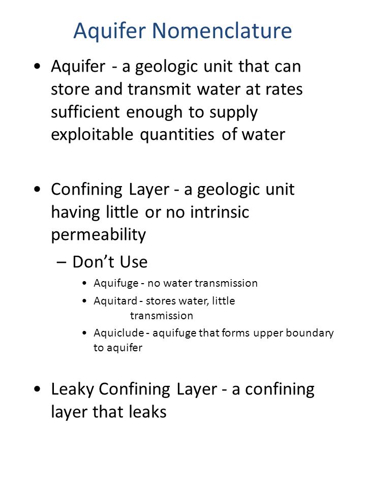
2. Aquifer Nomenclature Aquifer - a geologic unit that can store and transmit water at rates sufficient enough to supply exploitable quantities of water Confining Layer - a geologic unit having little or no intrinsic permeability –Don’t Use Aquifuge - no water transmission Aquitard - stores water, little transmission Aquiclude - aquifuge that forms upper boundary to aquifer Leaky Confining Layer - a confining layer that leaks

3. Types of Aquifers Rock Clay Sand K>>K’ K’<10 -7 Confined K = Horizontal Hydraulic Conductivity K’ = Vertical Hydraulic Conductivity Unconfined Sand Clay K’<<K K Leaky Confining Layer - Storage Ignored Semi-Confined Sand Clay K’<K K Real Leaky Confining Layer - Storage cannot be ignored Semi-Unconfined Sand

4. Perched Water Table

5. Unconfined Confined Water Table Potentiometric Surface Water Table Well Artesian Well Flowing Well The same aquifer can be both confined and unconfined.

6. Basic Hydraulic Parameters Soil Solid Water Air Vs = Vol of Solids Vw = Vol. of Water Va = Vol of Air Total Vol. (V t ) Va + Vw = Vv = Vol of Voids = Pore Space Variable No. 1 Porosity (n) = (Vv/Vt)x100 Expressed as %

7. Known Volume of Dry Soil Saturate Determining Porosity Volume of Water Added = Vol of Voids Example: 100 cm 3 soil, add 42 cm 3 water = 42% porosity Example: 1 m 2 10 m column Add 3 m of water to saturate soil What is porosity?

8. Variable No. 2 - Specific Yield Known Volume of Dry Soil Saturate Drain Volume Water Drained Total Volume Sample x 100 = Specific Yield (Sy) by Gravity

9. Volume Remaining on Soil Particles Total Volume = Specific Retention (Sr) Note: Specific Yield Dictates water bearing properties not porosity n = Sy + Sr Variable No. 3 – Specific Retention

10. Typical Values of n and Sy Unconsolidated n % Sy % Deposits Gravel 25 - 40 22 - 25 Sand 25 - 50 20 - 27 Silt 35 - 50 18 Clay 40 - 70 2 Rocks Primary n % Secondary n % sandstone 5 - 30 shale 0 - 10 crystalline < 5 Fractures increase overall n 2 to 5 % or more if weathered

12. Key Points Specific Yield is the Important Property for Flow Smaller the grain size – lower the Specific Yield n = Sy + specific retention Values usually estimated Porosity varies only over two orders of magnitude

13. Distribution of Water in Earth Materials Fluid Pressure: a. closed tube w/ sand b. saturated & sealed c. under pressure d. no flow - static Water in pore space exerts pressure on grains around pore space Define fluid pressure - P kg m/sec 2 P  Force/Unit Area = m 2 = N/m 2 = Pa Place Piezometer into tube to measure pressure A hphp “Water will rise in tube a height h p until Force produced by the weight of water in piezometer balances P being exerted in the pore space”

14. hphp P =  gh p  = density of water g = accel. of gravity h p = ht. of water in well Unit Weight Define -  g as unit weight - Force exerted by one unit volume of water  =  g  w = 9820 N/m 3 (metric) = 62.4 pcf (English) For water:

15. Typical Application clay A hphp P @A =  w h p Note: taking measurements of water levels in in a well provides more than P Unit Weight can be determined for anything -  d = dry unit weight - solids  b = bulk unit weight - solids + moisture  s = saturated unit weight - solids + water at saturation Typical Values Pierre shale - 90-100 pcf Sandy Gravel 8% moisture - 125-135 pcf Limestone - 165 pcf surface

16. Hydraulic Conductvity D constant head reservoir Measure Q L Sand datum h1h1 h2h2 Darcy’s Experiment (1857) hh Q   h Q   L Q  A

17. Pulling Terms Together Q  (  h/L) A Hydraulic Gradient (Slope of the fluid pressure term) hh L Slope = Hydraulic Gradient  h/L = I = dh/dL = i ft/ft or unitless Q/A gradient slope = K = Hydraulic Conductivity

18. Rewrite, Q = Darcy’s Law sometimes see it written with negative sign b/c flow is in the direction of decreasing fluid pressure - Units - m/sec, cm/sec, m/day, ft/day gpd/ft 2 1 Unit Volume 1 1 Conceptually, Gradient = 1 1 1 KIA K = Flow in gpd per unit area under unit hydraulic gradient @ 25 C°

19. Typical Values sandy gravel 10 -2 to 10 2 cm/sec silty clay 10 -6 to 10 -9 cm/sec Important Points to Remember: K varies over 12 to 14 orders of magnitude Major control on rate at which contaminants move in subsurface Main parameter needed in modeling Varies spatially in response to geology K1K1 K2K2 K3K3 K 2 > K 3 > K 1 contaminant Need to know how depositional/tectonic processes might influence spatial heterogeneity of K

20. Intrinsic Permeability Add Non-aqueous phase liquid D Measure Q L Sand datum h1h1 h2h2 hh Darcy’s Experiment Repeat Hold  h, L and A constant Q for water  Q for NAPL Q = KIA K must vary with fluid properties -

21. K  unit weight (  ) unit wt. = Force/unit volume =  g K   (density) K    (viscosity of fluid) Pulling terms together: K   g/  or K = k i  g/  Property of fluid Property of medium k i = intrinsic permeability - property of just the medium K = hydraulic conductivity - property of the medium and of fluid

22. Units for Intrinsic Permeability - cm 2, m 2, ft 2, etc Typical Values Material k i (cm 2 ) K (cm/sec) Clay 10 -12 to 10 -15 10 -6 to 10 -9 Silt or Till 10 -10 to 10 -12 10 -4 to 10 -6 Fine Sand 10 -9 to 10 -11 10 -3 to 10 -5 Well Sorted Sand 10 -7 to 10 -9 10 -1 to 10 -3 Well Sorted Gravel 10 -6 to 10 -8 10 0 to 10 -2 Define intrinsic permeability with lower case k with subscript i Hydraulic conductivity defined with a capital K Darcy’s Law Q = k i (  g/  ) (  h/L) A K

24. Key Points k i property of the medium only K a property of the medium and fluid K through identical material will vary with density, viscosity and temperature of fluid

25. Define Specific Storage Ss =  w g (   n  )  w = initial density of water g = acceleration due to gravity  n = porosity  = fluid compressibility = aquifer compressibility The volume of water either released from or taken into storage per unit volume of confined aquifer per unit change in fluid pressure Ss = Specific Storage

26. clay aquifer Conceptual meaning of Ss surface 1 unit vol Vol Out or In Ss = Volume of water released or taken into storage per unit volume of confined aq. 1 unit per unit head change in fluid pressure Units - m 3 /m 3 /m = 1/m so units of 1/L

27. clay aquifer surface 1 unit vol Vol Out or In 1 unit b b = aquifer thickness 1 unit area of aquifer Ss x b S = Ss x b Volume of water released or taken into storage from a vertical column of aquifer of height b, and unit basal area when subjected to a unit change in fluid pressure Storage Coefficient S is dimensionless

28. Transmissivity (T) surface clay aquifer b 1 unit vol I = 1 K K = volumetric flow per unit time per unit area of aquifer under a hydraulic gradient of one at 25 °C I = 1 K T T = volumetric flow per unit time per one unit width of the aquifer extended over the entire thickness of the aquifer at 25 °C K x b = T Units are: gpd/ft or m 3 /sec/m or m 2 /sec

29. Pumping a Confined Aquifer clay aquifer Q drop Aquifer is still saturated - how can this be?

30. Two Ways Water is Removed from Storage in a Confined Aquifer, water expands as it is released 1. Pumping decreases fluid pressure, so …... P ww VwVw Water Compressibility Component, water expelled by compression of aquifer 2. Pumping decreases fluid pressure, so …… P ee VtVt nstorage Aquifer Compressibility Summary - In a confined aquifer, water is released from storage by: 1. Expansion of water 2. Compression of the Aquifer

31. S is unitless Typical Values of S are 10 -3 to 10 -6 Removal of Water From Storage in an Unconfined Aquifer Surface P = 0 drop When you pump water out from an unconfined aquifer - you literally dewater the pore spaces Water drains by gravity - in accordance w/ Sy

32. Typical Values for Sy = 10 -1 to 10 -3 Storage actually = Sy + (Ss x b) Note: Usually neglect any aquifer compression or water expansion b/c Sy is so much larger S = Sy for an Unconfined Aquifer so, Key Points About Storage 1. Water released from storage in a confined aquifer by a) expansion of water and b) consolidation of aquifer material and is governed by S 2. Water is released from storage in an unconfined aquifer by dewatering the aquifer pores and is governed dominantly by Sy

33. clay aquifer Q drop Specific Capacity (SC) Pump well until steady drawdown in well is achieved Pumping Rate, Q / drawdown = Specific Capactiy Units are L 3 /T/L, eg., gal/day/ft,

34. General Relationship Between Specific Capacity and Transmissivity Transmissivity can be estimated by two empirical relationships and making some assumptions For a confined aquifer T = SC x 2000 Where, well radius = 0.5 feet pumping period = 1 day Initial T estimate = 30,000 gpd.ft Storage estimate = 10 -3 For an unconfined aquifer T = SC x 1500 Where, same as above except storage is 7.5 x 10 -2 Note: the effect of assuming a T value to estimate a T Value using this formula is not really a problem because It is derived from the Jacob modified non-equilibrium Equation and appears in a log term. So large variations In the assumed T has very little affect on the result.

35. Bedrock Aquifers Hydraulic Conductivity and Transmissivity of bedrock wells can also be determined through pumping tests Average K values can be determined for entire borehole T is determined by multiplying the average K value by the length of saturated uncased borehole length You can also set up packers and isolate individual water-bearing fractures to determine the K for an individual fracture

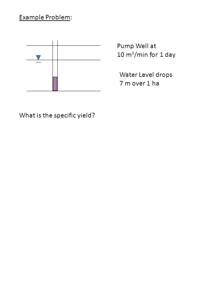
37. Example Problem: Pump Well at 10 m 3 /min for 1 day Water Level drops 7 m over 1 ha What is the specific yield?

38. Example Problem: Pump Well at 10 m 3 /min for 1 day Water Level drops 7 m over 1 ha What is the specific yield? 1. 10 m 3 /min x 60 min/hr x 24 hr/day x 1 day = 14400 m 3 2. 14400 m 3 /10000 m 2 = 1.44 m 3 /m 2 = 1.44 m = Volume of water extracted 3. Change in water level was 7 m or 7 m 3 /m 2 which is the total over which the change occurred 4. Therefore, 1.44/7 = 21 %

39. Tectonic Alluvial Valley Alternating layers of Sand, Silt, Clay

40. General Sequence polished bedrock Till veneer (lodgement or ablation or both Sand and Gravel Lacustrine Deposits Recent Deposits

41. surface P>0 Saturated Zone Ground- water P<0 Unsaturated Zone (Aeration or Vadose Zone) P=0 Water Table Phreatic Surface Capillary Zone Capillary Zone - combination of molecular attraction and surface tension between water and air capillarity Capillary zone can be saturated or nearly saturated but fluid pressure is negative soil-water (root) zone intermediate zone

42. Typical Water Profile in Soil 0 100% Saturation Depth (m) Water Table P=0 Saturated Zone Capillary Zone Tension Saturated Zone root zone intermediate zone Field Capacity (Specific Retention) PWP AWC Soil Moisture Recharge Happens

43. Importance of K and k i Distinction 1. Different fluids will travel at different rates Water and Non-Aqueous phase liquids will move at different rates due to differences in density and viscosity 2. Brines and highly saline solutions will move at different rates due to higher density of saline waters over fresh water. 3. Low temperature fluids will move at different rate than high temperature fluids Recall, viscosity and density are temperature dependent

44. Effective Stress & Storage Spring A z Spring = soil matrix Block of cement   = Total Stress (psf) Now let’s place the spring in a cell

45.  cell A imaginary piezometer closed h 1. fill to base of block 2. water represents fluid in pore spaces 3. no load carried by fluid Water rises in piezometer under its own weight - Hydrostatic Pressure P @A =  gh

46.  A h Place additional load on spring   1. Load applied matrix wants to consolidate and realign 2. Sealed tube, fluid has no where to go so additional load is borne by the fluid spring does not compress Excess fluid pressure 3. Additional load on fluid manifested in an increase in fluid pressure > hydrostatic z Start a Test

47.  h Drain   z 1. As water drains, excess fluid pressure dissipates 2. Load slowly transferred from fluid to matrix 3. Matrix responds by compressing - system consolidates and porosity decreases    z’ h

48. Fluid pressure returns to hydrostatic    z’’ h Aquifer is consolidated Total Stress,  t (  +   ) on system will resolve into 2 parts: P = Fluid Pressure load borne by the fluid  e = Effective Stress load borne by the solids  t =  e + P We write,

49.    z’ h Total Stress is balanced by load borne by the solids (  e ) and the load borne by the fluid (P) - At start of test, load borne by fluid - At completion of test load borne by solids - In between, load was shared by solids and fluid Excess Fluid Pressure During the Test

50. Behavior in Confined Aquifers surface clay aquifer Fluid Pressure Time rise + 0 fall - static Train clay

51. surface clay aquifer Fluid Pressure Time Train Train Stops rise + 0 fall - static clay Train leaves

52. Real Aquifers In real aquifers -  t (total stress) is constant Total stress never really changes so, if you increase P (fluid pressure) then you must reduce  e (effective stress) and vice versa So P and  e are the only parameters changing P +  e = constant  P   e so, Two Processes 1. Aquifer Compression place load on aquifer, matrix consolidates, reduces porosity, expells water ee, V t, n, Storage ee, V t, n, Storage

53. Aquifer Compressibility is:  = - (  V t / V to ) /  e 2. Water Compressibility increase pressure on water, volume will decrease, water will contract, density increases, more water can be stored P  Vw storage P Water Compressibility is:  = - (  V w / V wo ) /  P or since Mass is conserved, M =  w V w then  = (  w /  wo ) /  P  Vw storage

54. Fluid Pressure Time 1. Train approaches - total stress goes up - initially load carried by fluid - increase P Train Stops 2. Train stops - fluid pressure declines by draining rapid transfer from fluid to solids support - aquifer compresses by reducing porosity Train leaves 3. Train leaves - effective stress on solids released aquifer rebounds elastically and increases porosity - increase in pore volume lowers fluid pressure 4. Water flows back to low P zone - static rise + 0 fall - static

55. Geotechnical Application clay A surface  b = 100 pcf sand  s = 125 pcf 10 ft 5 ft Total Stress (Pressure) @ A = (100 pcf x 10 ft) + (125 pcf x 5 ft) = 1625 psf

56. Distribution of Water in Earth Materials – Saturated vs. Unsaturated surface water table 1. Take spot at 10 ft below water table Total P = Force/unit area from water + force/unit area atmosphere By convention, pressure at earth’s surface set is zero P =  w h p = 62.4 pcf x 10 ft Formal definition of the saturated zone - P > 0 Void space 100% saturated Vw/Vv = 1

57. surface water table 2. Take spot at 10 ft above water table Install tensiometer - surface tension and molecular attraction creates vacuum Soil Exerts tension which is negative Formal definition of the unsaturated zone - P < 0 Vw/Vv < 1 Voids do not have to be 100% saturated

58. surface water table 3. Take spot on the water table There is no column of water inside the piezometer exerting a force at water table Soil is saturated at the water table Formal definition of the water table - P = 0 Uniquely defines the water table

59. clay aquifer surface Storage Coefficient (S) b b = aquifer thickness 1 unit vol 1 unit area of aquifer Vol Out or In S = volume of water a confined aquifer releases or takes into storage per unit surface area of aquifer 1 unit per unit change in fluid pressure normal to that surface extended over the entire thickness of of the aquifer