1. Introduction to Logistic Regression

2. Content Simple and multiple linear regression Simple logistic regression –The logistic function –Estimation of parameters –Interpretation of coefficients Multiple logistic regression –Interpretation of coefficients –Coding of variables

3. Simple linear regression Table 1 Age and systolic blood pressure (SBP) among 33 adult women

4. SBP (mm Hg) Age (years) adapted from Colton T. Statistics in Medicine. Boston: Little Brown, 1974

5. Simple linear regression Relation between 2 continuous variables (SBP and age) Regression coefficient  1 –Measures association between y and x –Amount by which y changes on average when x changes by one unit –Least squares method y x Slope

6. Multiple linear regression Relation between a continuous variable and a set of i continuous variables Partial regression coefficients  i –Amount by which y changes on average when x i changes by one unit and all the other x i s remain constant –Measures association between x i and y adjusted for all other x i Example –SBP versus age, weight, height, etc

7. Multiple linear regression Dependent Independent variables Predicted Predictor variables Response variable Explanatory variables Outcome variable Covariables

8. Multivariate analysis Model Outcome Linear regression continous Poisson regression counts Cox model survival Logistic regression binomial...... Choice of the tool according to study, objectives, and the variables –Control of confounding –Model building, prediction

9. Logistic regression Models the relationship between a set of variables x i –dichotomous (eat : yes/no) –categorical (social class,... ) –continuous (age,...) and –dichotomous variable Y Dichotomous (binary) outcome most common situation in biology and epidemiology

10. Logistic regression (1) Table 2 Age and signs of coronary heart disease (CD)

11. How can we analyse these data? Comparison of the mean age of diseased and non-diseased women –Non-diseased: 38.6 years –Diseased: 58.7 years (p<0.0001) Linear regression?

12. Dot-plot: Data from Table 2

13. Logistic regression (2) Table 3 Prevalence (%) of signs of CD according to age group

14. Dot-plot: Data from Table 3 Diseased Age (years) P 1-P

15. Dot-plot: Data from Table 3 Diseased % Age (years)

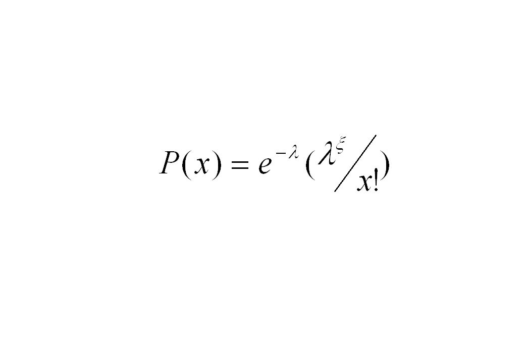
16. The logistic function (2) logit of P(y|x) {

17. The logistic function (3) Advantages of the logit –Simple transformation of P(y|x) –Linear relationship with x –Can be continuous (Logit between -  to +  ) –Known binomial distribution (P between 0 and 1) –Directly related to the notion of odds of disease

18. Interpretation of  (1)

19. Interpretation of  (2)  = increase in log-odds for a one unit increase in x Test of the hypothesis that  =0 (Wald test) Interval testing

20. Example Age (<55 and 55+ years) and risk of developing coronary heart disease (CD)

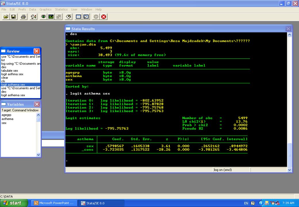
21. جمعپسردختر 18312459دارد 531628742442ندارد 549929982501جمع فراوانی مطلق ابتلا به آسم بر حسب جنس در دانش آموزان شهر زنجان 1374

22. پسردختر شيوع Odds لگاريتم Odds

24. Results of fitting Logistic Regression Model

25. Interpretation of  (1)

26. Multiple logistic regression More than one independent variable –Dichotomous, ordinal, nominal, continuous … Interpretation of  i –Increase in log-odds for a one unit increase in x i with all the other x i s constant –Measures association between x i and log-odds adjusted for all other x i

27. Multiple logistic regression Effect modification –Can be modelled by including interaction terms

28. Statistical testing Question –Does model including a given independent variable provide more information about dependent variable than model without this variable? Three tests –Likelihood ratio statistic (LRS) –Wald test

29. Fitting equation to the data Linear regression: Least squares Logistic regression: Maximum likelihood Likelihood function –Estimates parameters  and  with property that likelihood (probability) of observed data is higher than for any other values –Practically easier to work with log-likelihood

30. Likelihood ratio statistic Compares two nested models Log(odds) =  +  1 x 1 +  2 x 2 +  3 x 3 +  4 x 4 (model 1) Log(odds) =  +  1 x 1 +  2 x 2 (model 2)

31. Likelihood ratio statistic Compares two nested models Log(odds) =  +  1 x 1 +  2 x 2 +  3 x 3 +  4 x 4 (model 1) Log(odds) =  +  1 x 1 +  2 x 2 (model 2) LR statistic -2 log (likelihood model 2 / likelihood model 1) = -2 log (likelihood model 2) minus -2log (likelihood model 1) LR statistic is a  2 with DF = number of extra parameters in model

32. Example P Probability for cardiac arrest Exc 1= lack of exercise, 0 = exercise Smk 1= smokers, 0= non-smokers adapted from Kerr, Handbook of Public Health Methods, McGraw-Hill, 1998

33. Interactive effect between smoking and exercise? Product term  3 = -0.4604 (SE 0.5332) Wald test = 0.75 (1df) -2log(L) = 342.092 with interaction term = 342.836 without interaction term  LR statistic = 0.74 (1df), p = 0.39  No evidence of any interaction

34. Coding of variables (1) Dichotomous variables: yes = 1, no = 0 Continuous variables –Increase in OR for a one unit change in exposure variable –Logistic model is multiplicative  OR increases exponentially with x »If OR = 2 for a one unit change in exposure and x increases from 2 to 5: OR = 2 x 2 x 2 = 2 3 = 8 –Verify that OR increases exponentially with x. When in doubt, treat as qualitative variable

35. Continuous variable? Relationship between SBP>160 mmHg and body weight Introduce BW as continuous variable? –Code weight as single variable, eg. 3 equal classes: 40-60 kg = 0, 60-80 kg = 1, 80-100 kg = 2 –Compatible with assumption of multiplicative model –If not compatible, use indicator variables

36. Coding of variables (2) Nominal variables or ordinal with unequal classes: –Tobacco smoked: no=0, grey=1, brown=2, blond=3 –Model assumes that OR for blond tobacco = OR for grey tobacco 3 –Use indicator variables (dummy variables)

37. Indicator variables: Type of tobacco Neutralises artificial hierarchy between classes in the variable "type of tobacco" No assumptions made 3 variables (3 df) in model using same reference OR for each type of tobacco adjusted for the others in reference to non-smoking

38. تولد با وزن پايين (LBW) بعنوان يکي از شاخصهاي مهم سلامتي پيامدي است که شرايط اقتصادي و بهداشتي تاثير زيادي بر روي آن دارد. اين شرايط که به نوبه خود در مکانهاي مختلف متفاوتند باعث تنوع در الگوي مکاني رخداد تولد با وزن پايين مي شوند. توجه به اين جنبه و نقش پراهميت مکان در تنوع پيامدهاي بهداشتي حيطه اي است که در هر منطقه بايد جداگانه صورت گيرد تا مناطق پرخطر براي تخصيص مداخلات لازم شناسايي شوند. لذا اين بررسي با هدف تعيين مناطق پرخطر LBW در روستاهاي شهرستان رشت انجام شد.

39. روش كار: براي جمع آوري داده‌هاي اين مطالعه، تولدهاي با وزن زير 2500 گرم به تفکيک واحدهاي روستايي شهرستان رشت در فاصله زماني 1380 و 1381 از زيجهاي حياتي روستاها استخراج گرديد. براي تعيين توزيع مکاني تولدهاي با وزن پايين ابتدا "نقشه هاي مسطح" براي ميزان تولدهاي با وزن پايين تهيه شد.

40. تعداد كل LBW در روستاهاي شهرستان 295 مورد و تعداد زايمان‌هاي زنده 5987 است. آيا تعداد موارد LBW در روستاهاي زير بيش از حد انتظار شماست كد روستاتعداد تولد زنده LBW 8800800 8806322 8803361 8815361 8801244

42. محقق بر روي نقشه مناطق پر خطر LBW را مشخص مي‌كند. حال بنظرش مناسب مي‌رسد كه ارتباط برخي ازشاخصهاي بهداشتي و اقتصادي روستاها و تولد با وزن پايين را مورد سنجش قرار دهد. به همين دليل ميزان باروري عمومي(3/82)، دسترسي به خانه‌بهداشت(96 درصد) و دسترسي به وسيله نقليه در خانواده(52 درصد) را براي ساكنين روستاهاي شهرستان مشخص مي‌كند.

43. Poisson Regression Poisson Regression Analysis is used when the outcome variable comprises counts, usually of rather rare events e.g. number of cases of cancer over a defined period in a cohort of subjects. log (rate) = β0 + β1X1 + β2X2 + … +βnXn log (event/person-time) = β0 + β1X1 + … log (event) – log (person-time) = β0 + β1X1 + … log (event) = log (person-time) + β0 + β1X1 + … log (event) = β0* + β1X1 + …

44. شاخصضريب  محدوده اطمينان 95 درصد P value نداشتن خانه بهداشت 008/0-35/037/0-96/0 نداشتن آب لوله كشي 08/034/017/0-52/0 عدم دسترسي به وسايل نقليه 23/048/001/0-06/0 نداشتن مركز بهداشتي درماني 47/0-09/0-85/0-01/0 66-82 = GFR08/038/022/0-60/0 100-83 = GFR09/022/042/0-05/0

45. Reference Hosmer DW, Lemeshow S. Applied logistic regression.Wiley & Sons, New York, 1989

46. Example 1: Low Birth Weight Study 198 observations Low Birth Weigth [LBW] –1= Birth weight < 2500g –0= Birth weight >= 2500g Age of mother in years Weight of mother in pounds [LWT] Race (1,2,3) Number of doctor’s visit in last trimester [FTV]

47. Example 2: Risk of death from bacterial meningitis according to treatment 161 observations Death (0,1) Treatment –1=Chloramphenicol, 2=Ampicillin) Delay before treatment (onset, in days) Convulsions (1,0) Level of consciousness (1-3) Severity of dehydration (1-3) Age in years Pathogen –1 Others, 2 HiB, 3 Streptococcus pneumoniae

48. The logistic function (1) Probability of disease x

49. The logistic function (2) logit of P(y|x) {

50. Fitting equation to the data Linear regression: Least squares Logistic regression: Maximum likelihood Likelihood function –Estimates parameters  and  with property that likelihood (probability) of observed data is higher than for any other values –Practically easier to work with log-likelihood

51. Maximum likelihood Iterative computing –Choice of an arbitrary value for the coefficients (usually 0) –Computing of log-likelihood –Variation of coefficients’ values –Reiteration until maximisation (plateau) Results –Maximum Likelihood Estimates (MLE) for  and  –Estimates of P(y) for a given value of x