1. Maxwell’s Equations in Vacuum (1) .E =  /  o Poisson’s Equation (2) .B = 0No magnetic monopoles (3)  x E = -∂B/∂t Faraday’s Law (4)  x B =  o j +  o  o ∂E/∂t Maxwell’s Displacement Electric Field E Vm -1 Magnetic Induction B Tesla Charge density  Cm -3 Current Density Cm -2 s -1 Ohmic Conduction j =  E Electric Conductivity Siemens (Mho)

2. Constitutive Relations (1) D =  o E + P Electric Displacement D Cm -2 and Polarization P Cm -2 (2) P =  o  E Electric Susceptibility  (3)  =1+  Relative Permittivity (dielectric function)  (4) D =  o  E (5) H = B /  o – MMagnetic Field H Am -1 and Magnetization M Am -1 (6) M =  B  B /  o Magnetic Susceptibility  B (7)  =1 / (1-  B ) Relative Permeability  (8) H = B /   o  ~ 1 (non-magnetic materials),  ~ 1 - 50

3. Electric Polarisation Apply Gauss’ Law to right and left ends of polarised dielectric E Dep = ‘Depolarising field’ Macroscopic electric field E Mac = E + E Dep = E - P  o  ± surface charge density Cm -2  ± = P.n n outward normal E + 2dA =  + dA  o Gauss’ Law E + =  +  o E - =  -  o E Dep = E + + E - = (  +  -  o E Dep = -P/  o P =  + =  - -- E P ++ E+E+ E-E-

4. Electric Polarisation Define dimensionless dielectric susceptibility  through P =  o  E Mac E Mac = E – P/  o  o E =  o E Mac + P  o E =  o E Mac +  o  E Mac =  o (1 +  )E Mac =  o  E Mac Define dielectric constant (relative permittivity)  = 1 +  E Mac = E /  E =  E Mac Typical values for  : silicon 11.8, diamond 5.6, vacuum 1 Metal:  →∞ Insulator:  ∞ (electronic part) small, ~5, lattice part up to 20

5. Electric Polarisation Rewrite E Mac = E – P/  o as  o E Mac + P =  o E LHS contains only fields inside matter, RHS fields outside Displacement field, D D =  o E Mac + P =  o  E Mac =  o E Displacement field defined in terms of E Mac (inside matter, relative permittivity  ) and E (in vacuum, relative permittivity 1). Define D =  o  E where  is the relative permittivity and E is the electric field

6. Gauss’ Law in Matter Uniform polarisation → induced surface charges only Non-uniform polarisation → induced bulk charges also Displacements of positive charges Accumulated charges ++-- P - + E

7. Gauss’ Law in Matter Polarisation charge density Charge entering xz face at y = 0: P y=0  x  z Cm -2 m 2 = C Charge leaving xz face at y =  y: P y=  y  x  z = (P y=0 + ∂P y /∂y  y)  x  z Net charge entering cube via xz faces: (P y=0 - P y=  y )  x  z = -∂P y /∂y  x  y  z Charge entering cube via all faces: - (∂P x /∂x + ∂P y /∂y + ∂P z /∂z)  x  y  z = Q pol  pol = lim (  x  y  z)→0 Q pol /(  x  y  z) - . P =  pol xx zz yy z y x P y=  y P y=0

8. Gauss’ Law in Matter Differentiate - .P =  pol wrt time .∂P/∂t + ∂  pol /∂t = 0 Compare to continuity equation .j + ∂  /∂t = 0 ∂P/∂t = j pol Rate of change of polarisation is the polarisation-current density Suppose that charges in matter can be divided into ‘bound’ or polarisation and ‘free’ or conduction charges  tot =  pol +  free

9. Gauss’ Law in Matter Inside matter .E = .E mac =  tot /  o = (  pol +  free )/  o Total (averaged) electric field is the macroscopic field - .P =  pol .(  o E + P) =  free .D =  free Introduction of the displacement field, D, allows us to eliminate polarisation charges from any calculation. This is a form of Gauss’ Law suitable for application in matter.

10. Ampère’s Law in Matter Ampère’s Law Problem! A steady current implies constant charge density, so Ampère’s law is consistent with the continuity equation for steady currents Ampère’s law is inconsistent with the continuity equation (conservation of charge) when the charge density is time dependent Continuity equation

11. Ampère’s Law in Matter Add term to LHS such that taking Div makes LHS also identically equal to zero: The extra term is in the bracket extended Ampère’s Law Displacement current (vacuum)

12. Ampère’s Law in Matter Polarisation current density from oscillation of charges in electric dipoles Magnetisation current density variation in magnitude of magnetic dipoles M = sin(ay) k k i j j M = curl M = a cos(ay) i Total current

13. Ampère’s Law in Matter ∂D/∂t is the displacement current postulated by Maxwell (1862) In vacuum D =  o E ∂D/∂t =  o ∂E/∂t In matter D =  o  E ∂D/∂t =  o  ∂E/∂t Displacement current exists throughout space in a changing electric field

14. Maxwell’s Equations in vacuum in matter .E =  /  o .D =  free Poisson’s Equation .B = 0 .B = 0 No magnetic monopoles  x E = -∂B/∂t  x E = -∂B/∂t Faraday’s Law  x B =  o j +  o  o ∂E/∂t  x H = j free + ∂D/∂t Maxwell’s Displacement D =  o  E =  o (1+  )EConstitutive relation for D H = B/(  o  ) = (1-  B )B/  o Constitutive relation for H

15. Divergence Theorem 2-D 3-D From Green’s Theorem In words - Integral of A.n dA over surface contour equals integral of div A over surface area In 3-D Integral of A.n dA over bounding surface S equals integral of div V dV within volume enclosed by surface S The area element n dA is conveniently written as dS A.n dA .A dV

16. Differential form of Gauss’ Law Integral form Divergence theorem applied to field V, volume v bounded by surface S Divergence theorem applied to electric field E V.dS .V dv Differential form of Gauss’ Law (Poisson’s Equation)

17. Stokes’ Theorem 3-D In words - Integral of (  x A).n dA over surface S equals integral of A.dr over bounding contour C It doesn’t matter which surface (blue or hatched). Direction of dr determined by right hand rule. (  x a).ndA n outward normal dA local value of  x A local value of A drdr A. drA. dr A C

18. Faraday’s Law

19. Integral form of law: enclosed current is integral dS of current density j Apply Stokes’ theorem Integration surface is arbitrary Must be true point wise Differential form of Ampère’s Law S j B dℓdℓ

20. Maxwell’s Equations in Vacuum Take curl of Faraday’s Law (3)  x (  x E) = -∂ (  x B)/∂t = -∂ (  o  o ∂E/∂t)/∂t = -  o  o ∂ 2 E/∂t 2  x (  x E) =  ( .E) -  2 E vector identity -  2 E = -  o  o ∂ 2 E/∂t 2 ( .E = 0)  2 E -  o  o ∂ 2 E/∂t 2 = 0 Vector wave equation

21. Maxwell’s Equations in Vacuum Plane wave solution to wave equation E(r, t) = Re {E o e i (  t - k.r) }E o constant vector  2 E =(∂ 2 /∂x 2 + ∂ 2 /∂y 2 + ∂ 2 /∂z 2 )E = -k 2 E .E = ∂E x /∂x + ∂E y /∂y + ∂E z /∂z = - i k.E = - i k.E o e i (  t - k.r) If E o || k then .E ≠ 0 and  x E = 0 If E o ┴ k then .E = 0 and  x E ≠ 0 For light E o ┴ k and E(r, t) is a transverse wave

22. r r || rr k Consecutive wave fronts Plane waves travel parallel to wave vector k Plane waves have wavelength 2  /k Maxwell’s Equations in Vacuum EoEo

23. Plane wave solution to wave equation E(r, t) = E o e i (  t - k.r) E o constant vector  o  o ∂ 2 E/∂t 2 = -  o  o  2 E  o  o  2 = k 2  =±k/(  o  o ) 1/2 = ±ck  /k = c = (  o  o ) -1/2 phase velocity  = ±ck Linear dispersion relationship  (k) k

24. Maxwell’s Equations in Vacuum Magnetic component of the electromagnetic wave in vacuum From Maxwell-Ampère and Faraday laws  x (  x B) =  o  o ∂(  x E)/∂t =  o  o ∂(-∂B/∂t)/∂t = -  o  o ∂ 2 B/∂t 2  x (  x B) =  ( .B) -  2 B -  2 B = -  o  o ∂ 2 B/∂t 2 ( .B = 0)  2 B -  o  o ∂ 2 B/∂t 2 = 0 Same vector wave equation as for E

25. Maxwell’s Equations in Vacuum If E(r, t) = E o e x e i (  t - k.r) and k || e z and E || e x (e x, e y, e z unit vectors)  x E = - i k E o e y e i (  t - k.r) = -∂B/∂t From Faraday’s Law ∂B/∂t = i k E o e y e i (  t - k.r) B = (k/  ) E o e y e i (  t - k.r) = (1/c) E o e y e i (  t - k.r) For this wave E || e x, B || e y, k || e z, cB o = E o More generally -∂B/∂t = - i  B =  x E  x E = - i  k x E - i  B = - i  k x E B = e k x E / c exex eyey ezez

26. Maxwell’s Equations in Matter Solution of Maxwell’s equations in matter for  = 1,  free  = 0, j free = 0 EM wave in a dielectric with frequency at which dielectric is transparent Maxwell’s equations become  x E = -∂B/∂t  x H = ∂D/∂t H = B /  o D =  o  E  x B =  o  o  ∂E/∂t  x ∂B/∂t =  o  o  ∂ 2 E/∂t 2  x (-  x E) =  x ∂B/∂t =  o  o  ∂ 2 E/∂t 2 -  ( .E) +  2 E =  o  o  ∂ 2 E/∂t 2 .  E = . E = 0 since  free  = 0  2 E -  o  o  ∂ 2 E/∂t 2 = 0

27. Maxwell’s Equations in Matter  2 E -  o  o  ∂ 2 E/∂t 2 = 0 E(r, t) = E o e x Re{e i (  t - k.r) }  2 E = -k 2 E  o  o  ∂ 2 E/∂t 2 = -  o  o  2 E (-k 2  +  o  o  2 )E = 0  2 = k 2 /(  o  o  )  o  o   2 = k 2 k = ±  √(  o  o  ) k = ± √   /c Let  =  1  - i  2  be the real and imaginary parts of  and  = (n  - i  ) 2 We need √  = n  - i   = (n  - i  ) 2 = n 2  -  2 - i 2n   1  = n 2  -  2  2  = 2n  E(r, t) = E o e x Re{ e i (  t - k.r) } = E o e x Re{e i (  t - kz) } k || e z = E o e x Re{e i (  t - (n - i  )  z/c) } = E o e x Re{e i (  t - n  z/c) e -  z/c) } Attenuated wave with phase velocity v p = c/n

28. Maxwell’s Equations in Matter Solution of Maxwell’s equations in matter for  = 1,  free  = 0, j free =  (  )E EM wave in a metal with frequency at which metal is absorbing/reflecting Maxwell’s equations become  x E = -∂B/∂t  x H = j free + ∂D/∂t H = B /  o D =  o  E  x B =  o j free +  o  o  ∂E/∂t  x ∂B/∂t =  o  ∂E/∂t +  o  o  ∂ 2 E/∂t 2  x (-  x E) =  x ∂B/∂t =  o  ∂E/∂t +  o  o  ∂ 2 E/∂t 2 -  ( .E) +  2 E =  o  ∂E/∂t +  o  o  ∂ 2 E/∂t 2 .  E = . E = 0 since  free  = 0  2 E -  o  ∂E/∂t -  o  o  ∂ 2 E/∂t 2 = 0

29. Maxwell’s Equations in Matter  2 E -  o  ∂E/∂t -  o  o  ∂ 2 E/∂t 2 = 0 E(r, t) = E o e x Re{e i (  t - k.r) } k || e z  2 E = -k 2 E  o  ∂E/∂t =  o  i  E  o  o  ∂ 2 E/∂t 2 = -  o  o  2 E (-k 2  -  o  i  +  o  o  2 )E = 0  o  for a good conductor E(r, t) = E o e x Re{ e i (  t - √(  o / 2 )z) e -√(  o / 2 )z } NB wave travels in +z direction and is attenuated The skin depth  = √(2/  o ) is the thickness over which incident radiation is attenuated. For example, Cu metal DC conductivity is 5.7 x 10 7 (  m) -1 At 50 Hz  = 9 mm and at 10 kHz  = 0.7 mm

30. Bound and Free Charges Bound charges All valence electrons in insulators (materials with a ‘band gap’) Bound valence electrons in metals or semiconductors (band gap absent/small ) Free charges Conduction electrons in metals or semiconductors M ion k m electron k M ion Si ion Bound electron pair Resonance frequency  o ~ (k/M) 1/2 or ~ (k/m) 1/2 Ions: heavy, resonance in infra-red ~10 13 Hz Bound electrons: light, resonance in visible ~10 15 Hz Free electrons: no restoring force, no resonance

31. Bound and Free Charges Bound charges Resonance model for uncoupled electron pairs M ion k m electron k M ion

32. Bound and Free Charges Bound charges In and out of phase components of x(t) relative to E o cos(  t) M ion k m electron k M ion in phase out of phase

33. Bound and Free Charges Bound charges Connection to  and       Im{  } Re{  }

34. Bound and Free Charges Free charges Let   → 0 in  and  j pol = ∂P/∂t     Im{  }  Re{  } Drude ‘tail’

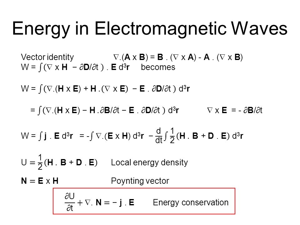
35. Energy in Electromagnetic Waves

37. Energy density in plane electromagnetic waves in vacuum