1. MPO 674 Lecture 22 4/2/15

2. Single Observation Example for 4D Variants D. Kleist et al. 4DVAR H-4DVAR_AD  f -1 =0.25 H-4DENVAR  f -1 =0.25 4DENVARTLMADJ ENSONLY

3. Synop: 450,000 0.3% Aircraft: 434,000 0.3% Dribu: 24,000 0.02% Temp: 153,000 0.1% Pilot: 86,000 0.1% AMV’s: 2,535,000 1.6% Radiance data: 150,663,000 96.9% Scat: 835,000 0.5% GPS radio occult. 271,000 0.2% TOTAL: 155,448,000 100.00% Synop: 64,000 0.7% Aircraft: 215,000 2.4% Dribu: 7,000 0.1% Temp: 76,000 0.8% Pilot: 39,000 0.4% AMV’s: 125,000 1.4% Radiance data: 8,207,000 91.0% Scat: 149,000 1.7% GPS radio occult. 137,000 1.5% TOTAL: 9,018,000 100.00% Screened Assimilated 99% of screened data is from satellites 96% of assimilated data is from satellites Observation data count for one 12h 4D-Var cycle 0900-2100UTC 3 March 2008

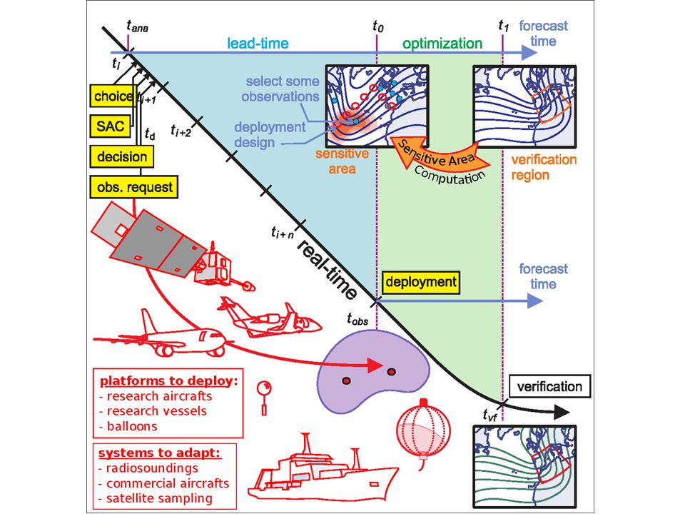
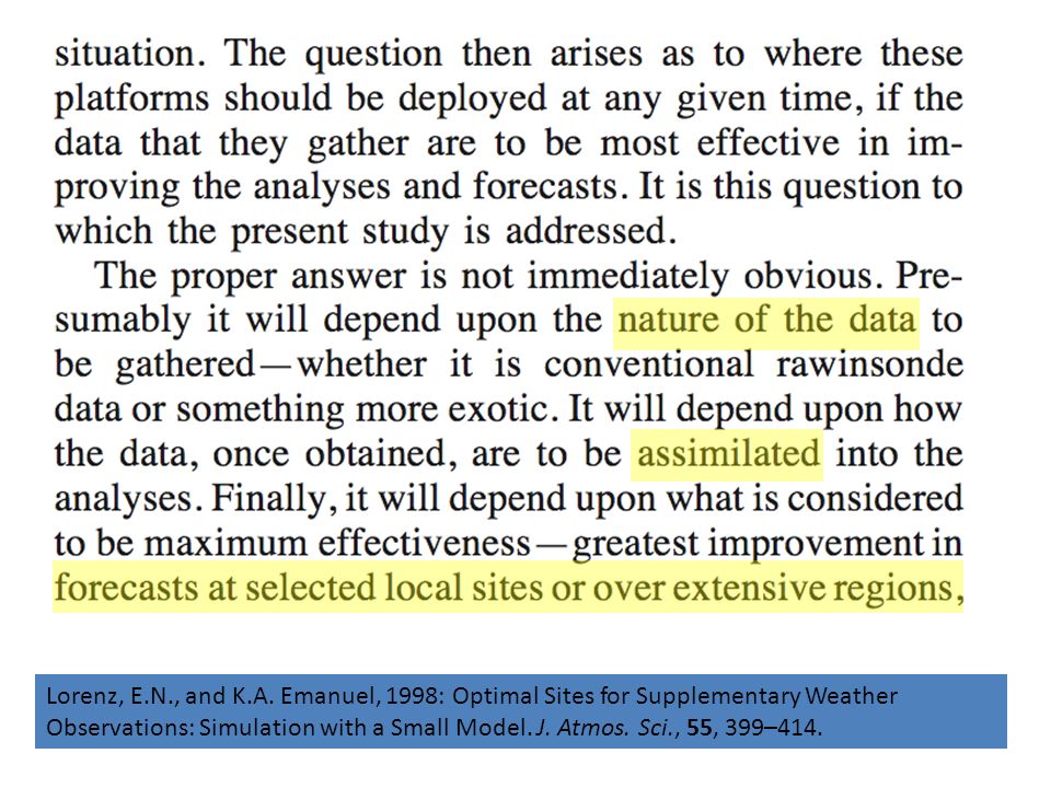
4. Lorenz, E.N., and K.A. Emanuel, 1998: Optimal Sites for Supplementary Weather Observations: Simulation with a Small Model. J. Atmos. Sci., 55, 399–414.

7. UYonsei MM5SVNRL SVJMA SV ECMWF SVUMiami-NCEP ETKFUKMO ETKF Targeted observing guidance (Typhoon Sinlaku, 2008)

8. Sensitivity Methods Observation sensitivity – ETKF – Adjoint Observation Sensitivity / Impact Analysis sensitivity – Singular Vectors (done) – Adjoint Sensitivity (done) – Ensemble Sensitivity

9. Signals and Signal Variance Squared NCEP MRF signal 1/2 (u’ 2 +v’ 2 ) + (c p /T r ) T’ 2 valid at analysis time t a Predicted ETKF signal variance S q, using ensembles initiated 36h prior to analysis time t a

10. tata tata ETKF Summary map of Signal Variance S q, for many different q. Summary bar chart tvtv tvtv GoodPoor Aim: to improve a 24-hr forecast on the West Coast

11. Evolution of operational signal over 84h

12. Evolution of predicted ETKF signal variance over 84h

14. Signal realization versus forecast error reduction, at verification time t v

15. 0ld method: ETKF-based P r Heavy emphasis on TC (obvious target) Secondary targets in areas of high ensemble variance over ocean, downstream of TC

16. New method: Ensemble transform based on operational analysis error variance Less emphasis on TC Secondary targets: often upstream, in subtropical jet and mid- latitude troughs

17. Suppose we wish to sample through 4 days of Typhoon Ewiniar (2006) as it recurves. Can one identify spatio-temporal continuity of ETKF target regions? Extension into medium-range (forecasts beyond 2 days)

18. -4 days

19. -3.5 days

20. -3 days

21. -2.5 days

22. -2 days

23. -1.5 days

24. -1 day

25. -0.5 days

26. 0 days

27. Serial adaptive sampling Many combinations and permutations of adaptive observations are available. Suppose that two sets of observations can be deployed simultaneously. First, find the optimal first deployment. Next, calculate the best second deployment given that the first set of observations are to be assimilated by the ETKF at the same time. Reduces observational redundancy.

28. Flight track number Serial adaptive sampling during Winter Storm Reconnaissance

29. Shortcomings of ETKF targeting strategy Inconsistency between imperfect error covariance in ETKF and operational data assimilation scheme Limited # ensemble members gives a rank-deficient P : leads to spurious correlations Ensemble mean and variance predictions must be reasonably accurate Theory is (quasi) linear

30. Dependence of SVs on the analysis-time norm: Hurricane Charley (2004) Using NAVDAS analysis error variance as constraint pushes primary target northward into Canada. 2-day growth diminished from 54.4 to 36.4. NOGAPS Total-Energy SV NOGAPS Variance SV NAVDAS Analysis Error Variance Reynolds

31. Ensemble Sensitivity (from Ryan Torn)

32. Overview Want to understand how initial condition errors associated with vortex and environment regulate the predictability of TC genesis Focus on two forecasts initialized roughly 48 h prior to genesis, one for Karl and another for Danielle R. Torn

33. Karl Forecast R. Torn

34. Methods Use ensemble-based sensitivity analysis to compute the sensitivity of 48 h 850 hPa circulation associated with the pre-genesis system to the initial conditions R. Torn

35. Sensitivity R. Torn Sensitivity of 48-h 850 hPa circ to 0-h 850 hPa circ Sensitivity of 48-h 850 hPa circ to 0-h 400 hPa theta-e

36. Vortex Sensitivity Most of the sensitivity appears to be associated with the pre-genesis system itself Instead compute sensitivity of forecast to vortex-average quantities at each vertical level for different lead times. R. Torn

37. Vortex Sensitivity R. Torn

38. Upwind Moisture Sensitivity Interesting to see the sensitivity of upwind moisture to the initial moisture field Compute sensitivity as before, except metric is now 0-48 h upwind moisture in 400-600 hPa layer R. Torn

39. Upwind Moisture Sensitivity R. Torn

40. Danielle Forecast R. Torn

41. Danielle Sensitivity R. Torn Sensitivity of 48-h 850 hPa circ to 0-h 850 hPa circ Sensitivity of 48-h 850 hPa circ to 0-h 400 hPa theta-e Increase theta-e to the south  stronger circulation Decrease theta-e to the north  stronger circulation

42. Danielle Sensitivity R. Torn Forecast of pre-Danielle has less “memory” of the initial vortex than Karl. Lower-level sensitivity of q and theta-e.