1. A brief introduction to phylogenetics

2. Genetic Distance Definition:
The number of evolutionary events (usually nucleotide substitutions) that have occurred since two sequences diverged from a common ancestor
Simplest distance: p-distance
= proportion of sites that are different

3. A T T G C G C A T T G C G C Correcting for ‘multiple substitutions’ C
Differences

4. Correcting for multiple substitutions
Requires a statistical ‘model’ of how the process of substitution works to correct for
Differences in the rates of different substitution types (e.g. Jukes and Cantor – all substitutions are treated the same versus Kimura 2-parameter model – distinguishes between transitions and transversions)
Different frequencies of different nucleotides (e.g. GC content – the HKY model adds nucleotide frequency parameters to the Kimura 2-parameter model)
Different rates at different sites (often modelled using a distribution – e.g. Gamma distribution – see next)

5. In order to perform a gamma correction for site specific rates you need to know the shape of the gamma distribution

6. Correcting for multiple substitutions (continued…)
Correction for multiple substitutions implies a model of evolution, but some models have many more parameters than others
- Models with few parameters are easy to fit, but may miss some important biology (e.g. there’s typically a big difference between rates of transition and transversion, and it would be dangerous not to model that). Simple models can underfit the data.
- Complex models (many parameters) may be difficult and much slower to estimate. There can also be a danger of over-fitting the data when more parameters are included in a model than are necessary.
(see later…)

7. - genetic distances can be far greater than 1
Some general points:
- genetic distances can be far greater than 1
- smaller genetic distances are more reliable
- model choice has a bigger impact for distantly related sequences
- normally positions with gaps are ignored (complete deletion)
- IF you know the rate of evolution for a pair of sequences (and if the rate has remained more or less constant) you can estimate the date at which they diverged

8. Phylogenetic tree Diagram consisting of branches and nodes
Branches indicate relationships between the ‘objects’
Internal branches define partitions of the objects

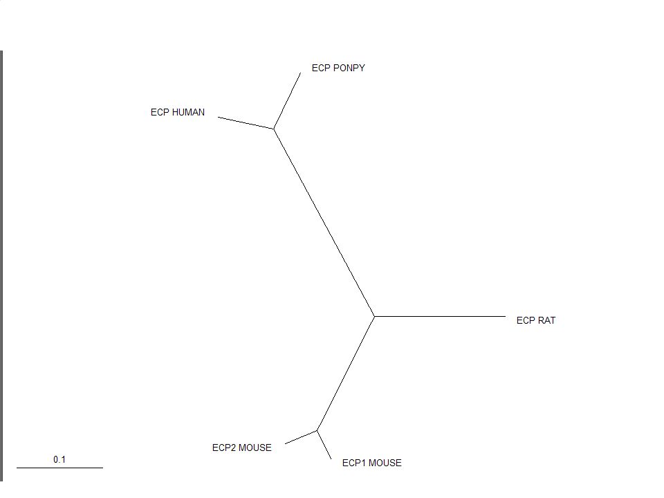
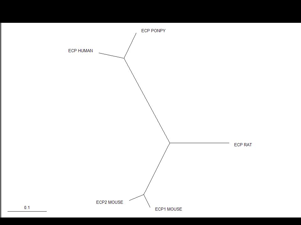
10. Rooting the Tree
In an unrooted tree the direction of evolution is unknown
The root is the hypothesized ancestor of the sequences in the tree
The root can either be placed on a branch or at a node
You should start by viewing an unrooted tree

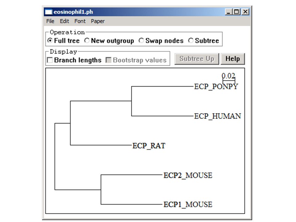
13. Many software packages will root trees automatically (e. g
Many software packages will root trees automatically (e.g. mid-point rooting in NJPlot)
This always involves assumptions… BEWARE!

14. Rooting Using an Outgroup
1. The outgroup should be a sequence (or set of sequences) known to be less closely related to the rest of the sequences than they are to each other
2. It should ideally be as closely related as possible to the rest of the sequences while still satisfying condition 1
The root must be somewhere between the outgroup and the rest (either on the node or in a branch)

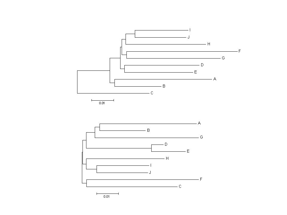
15. Sometimes two trees may look very different but, in fact, differ only in the position of the root

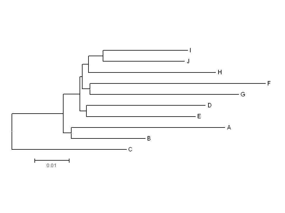
16. Looking at trees
Two trees are different if one tree specifies at least one partition that is not present in the other

21. Phylogenetic Inference
Distance, parsimony and maximum likelihood methods

22. need
optimality criteria +
algorithm to search for the best tree given the optimality criteria

23. Best tree Vs True tree

24. Types of optimality criteria used to infer phylogeny from sequence
Distance methods
Parsimony
Likelihood
Others

25. Distance based methods
Minimum Evolution Principal
“The tree with the smallest sum of branch lengths is the best tree”

26. Tree length = u + v + t + r + sA B r s t u v D C
dAB ~ r + s
dCD ~ u + v
dAD ~ r + t + v
dBC ~ s + t + u
etc.
(r, s, u, v, t are estimated so that these relationships are as close as possible to being correct)
Tree length = u + v + t + r + s

27. Number of possible unrooted trees from n sequences:
e.g. for 20 sequences there are approximately 1020

28. For realistic numbers of sequences it is impossible to consider all possible trees.
Need algorithms that can arrive at the ‘best tree’ without considering all possible trees.

29. Neighbour joining is a very fast approximation to minimum evolution

30. Neighbour Joining 8 8 7 6 5 2 3 4 1 7 1 2 6 3 5 4
Choose the pair that minimizes the length of the resulting tree

31. Maximum Parsimony Occam’s Razor
Entia non sunt multiplicanda praeter necessitatem.
William of Occam ( )
The best tree is the one which requires the least number of substitutions

32. Check each topology
Count the minimum number of changes required to explain the data
Choose the tree with the smallest number of changes
Usually performs well with closely related sequences – but often performs badly with very distantly related sequences
With distantly related sequences homoplasy becomes a major problem

33. Informative sites: Not all sites contain information about the tree topology using the parsimony approach
Homoplasy: characters that are similar for reasons other than common ancestry (increasingly a problem as sequences become more divergent)

34. Methods for searching for the ‘best’ tree without considering all trees
Branch & Bound: A method that does not have to consider all trees but still guarantees finding the ‘best’ tree. Slow for large numbers of sequences.
Heuristic methods (No guarantee of finding the best tree)
- Start with some tree (e.g. the neighbour-joining tree)
- Consider making a random change to the tree
- make the change if it improves the score of the tree
- stop making changes when you can find no further improvement
NNI -> SPR -> TBR
(NNI fastest and least rigorous, TBR slowest and most rigorous)

35. How confident are we that the tree is correct?
Bootstrap values
Bootstrapping is a statistical technique that can use random resampling of data to determine sampling error for tree topologies

36. Bootstrapping phylogenies
Characters are resampled with replacement to create many bootstrap replicate data sets
Each bootstrap replicate data set is analysed (e.g. with parsimony, distance, ML etc.)
Agreement among the resulting trees is summarized with a majority-rule consensus tree
Frequencies of occurrence of groups, bootstrap proportions (BPs), are a measure of support for those groups

38. Bootstrap - interpretation
Bootstrapping is a very valuable and widely used technique (it is demanded by some journals)
BPs give an idea of how likely a given branch would be to be unaffected if additional data, with the same distribution, became available
BPs are not the same as confidence intervals. There is no simple mapping between bootstrap values and confidence intervals. There is no agreement about what constitutes a ‘good’ bootstrap value (> 70%, > 80%, > 85% ????)
Some theoretical work indicates that BPs can be a conservative estimate of confidence

39. Inferring trees using Likelihood

40. The ‘optimality criterion’
The best tree is the one that makes the data have the highest likelihood
The ML optimality criterion will lead to the correct tree given
- enough data (e.g. long enough sequence alignment)
- the correct model (e.g. Kimura 2 parameter model)

41. A C G
G A G
Suppose we have a model of evolution (e.g. Jukes & Cantor) that allows us to work out the probability of each pair of characters, given a particular genetic distance (c.f. series of scoring matrices like BLOSUM, PAM etc)
Distance
Likelihood
D = 0.3
L = 0.06
D = 0.6
0.6 * 0.6 * 0.4 = 0.144
D = 0.9
0.9 * 0.9 * 0.1 = 0.081

42. Genetic Distance using Maximum Likelihood
Require a model of evolution
Optimise all parameters of the model
Each evolutionary ‘event’ has an associated likelihood given an inferred genetic distance
The likelihood of the sequence-pair is a function of the genetic distance (just the product of the likelihoods of each of the inferred ‘events’ at each sequence position)
Function is maximized

43. Phylogenetic trees using Maximum Likelihood
Require a model of evolution
Each substitution has an associated likelihood given a branch of a certain length
A function is derived to represent the likelihood of the data given the tree, branch-lengths and additional parameters
Optimise over parameters of the model
Optimise over branch lengths
Sum the likelihood over all possible sequences at ancestral nodes
Search for the best tree (using heuristics such as TBR)

44. Models can be made more parameter rich to increase their realism
The most common additional parameters are:
A correction to allow different rates for each type of nucleotide change
Parameters for equilibrium base frequencies
A correction for the proportion of sites which are unable to change
A correction for variable rates at those sites which can change
The values of the additional parameters will be estimated in the process

45. Likelihood and the number of parameters
More parameters always leads to a better fit of the data

46. Likelihood and the number of parameters
More parameters always leads to a better fit of the data

47. More parameters always leads to a higher value of the likelihood whether or not the additional parameters are providing a ‘significantly’ better fit to the data

48. ( ) Likelihood ratio statistic: 2 log
Are the extra parameters justified?
- Likelihood ratio test (
Maximum Likelihood | H1 )
Likelihood ratio statistic: log
Maximum Likelihood | H0
Has chi-squared distribution
dof = number of additional parameters

49. One model is nested in another if it is a special case of the more general model
e.g. the Jukes and Cantor model and Kimura 2P model
J-C
K2P

50. Modeltest
- Uses PAUP
- Tries out many nested models of nucleotide substitution
- Decides how many parameters are justified by the data
GTR does not overfit the data for at least some HIV sequences

51. Bayesian methods

52. The ‘optimality criterion’
The best tree is the one that has the highest probability of being the true tree

53. Likelihood: Choose the tree that makes the data the most likely
Bayesian: Choose the most probable tree (tree with the highest posterior probability)
Equivalent to maximizing
Equivalent to maximizing

54. Bayes’ Rule Probability = Likelihood X Prior Information
Some normalising factors
Mathematically:
T = Tree
D = Data

55. Important Terms
Prior probability: the probability of the event before considering the data
Posterior probability: the probability of the event after taking the data into consideration

56. In molecular phylogenetics the prior is usually ‘flat’ so the max likelihood tree is usually also the max probability tree
So why bother?

57. 1. Because we get the answer as a probability
2. Because this formulation allows us to use another approach to get to the best tree (MCMC – see later)
3. Also allows us to integrate over parameters instead of optimising over parameters

58. MCMC (Markov Chain Monte Carlo)
Produces a long chain of trees/parameters sampled according to their probability
The number of times the chain visits tree X is proportional to the probability of tree X

59. Burnin
Typically the chain will take some time before trees are sampled according to their probability
Initially probability of trees increases with time
Programmes need to be allowed to run until the probabilities are fluctuating randomly about a constant mean
Data generated before the chain reaches a steadystate are discarded

60. Bayesian methods can be
- relatively fast
- easily interpretable
- often very accurate

61. But
- sometimes overestimate confidence
- difficult to be sure of convergence (less of a problem with more recent software versions)
=> difficult to decide how long to run the chain
Software for Bayesian phylogenetics: MrBayes