1. Ch. 6-7– Routing Theory – Part 3 CCNA Semester 2 Originally by Rick Graziani, Instructor Modified by Prof. Yousif

4. Link-State Routing Protocols The first type of routing protocol we discussed was distance vector. The second type of routing protocol that we will examine is link-state. In this presentation we will only examine the very basic concepts of link-state routing protocols. In CCNP Advanced Routing we examine the link state routing protocol OSPF in detail. I have added a presentation, Introduction to OSPF, which we will discuss at the end of this semester.

5. Distance Vector Routing Protocols Distance vector routing protocols like RIP and IGRP do not know the exact topology of a network. All distance vector routing decisions are made from information from neighboring routers – routing by rumor. The only information the router has about a route is how far away the network is in hops or using another cost (distance) and which interface to send forward the packet out of (vector). The router has no way to make its own decision on which direction is ultimately the best way to send the packets.

6. Link-State Routing Protocols - History An IETF working group designed a routing protocol specifically for IP routing, OSPF (Open Shortest Path First). For most network administrators they had two open-standard routing protocols to choose from: RIP, simple but very limited, or OSPF, robust but more sophisticated to implement. –IGRP and EIGRP are Cisco proprietary –IS-IS is used in IP networks, but not as common as OSPF

7. Theory of Link-State Routing Protocols In this presentation we will examine “some” of the theory behind link- state routing protocols. This will only be a brief introduction to the link-state theory, requiring much more time and perhaps even some requisite knowledge of algorithms. At the end of this presentation will be some suggested resources for leaning more about the theory of link-state routing and Dijkstra’s algorithm.

8. Mathematical point of view Link-state routing is not based on IP addresses, subnets and network information! Link-state routing has a mathematical point of view, looking at the network as nothing more than a graph with vertices and the costs to these vertices. Okay, I’m losing you and I said I wouldn’t get mathematical. Link-state routing is based on a very simple algorithm known as Dijkstras’s algorithm, invented by Edsger Wybe Dijkstra This algorithm can and has been used in many areas of human activity, not just for routing.

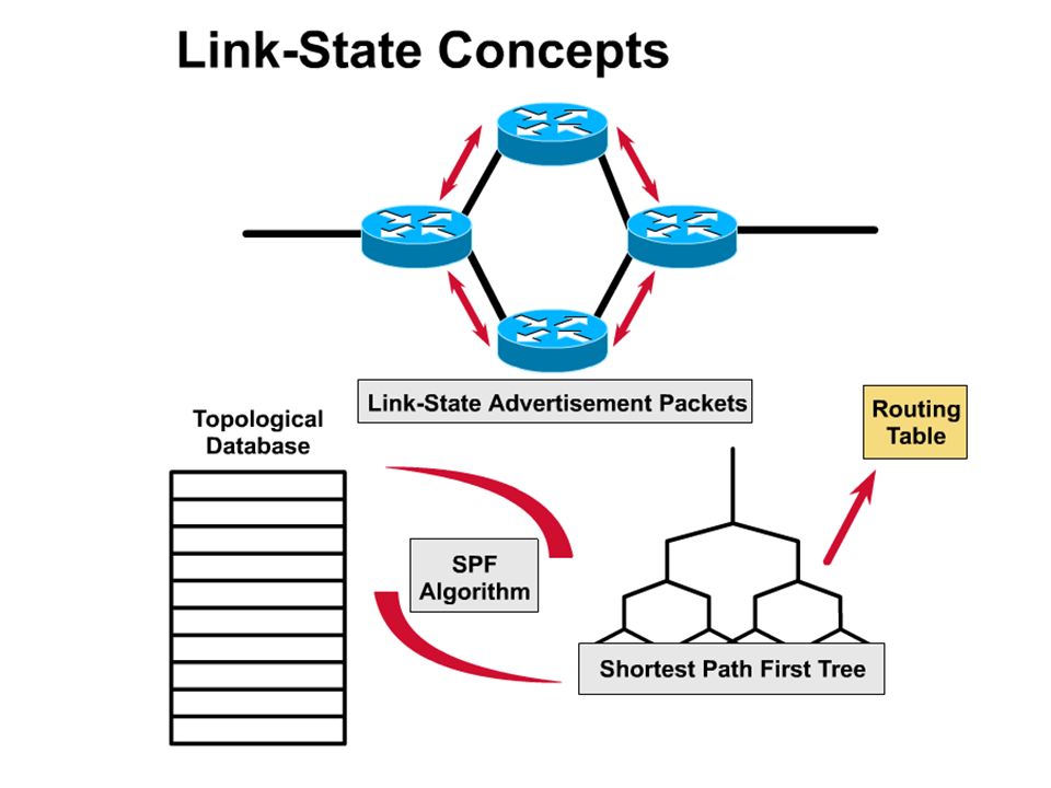
9. Link-State Theory The network is viewed as a graph, showing the complete topology of the network. How do routers build this topology? 1 – Flooding of link-state information The first thing that happens is that each node, router, on the network announces its own piece of link-state information to other all other routers on the network: who their neighboring routers are and the cost of the link between them. Example: “Hi, I’m RouterA, and I can reach RouterB via a T1 link and I can reach RouterC via an Ethernet link.” Each router sends these announcements to all of the routers in the network. 1 – Flooding of link-state information

10. 2. Building a Topological Database Each router collects all of this link-state information from other routers and puts it into a topological database. 3. Shortest-Path First (SPF), Dijkstra’s Algorithm Using this information, the routers can recreate a topology graph of the network. Believe it or not, this is actually a very simple algorithm and I highly suggest you look at it some time, or even better, take a class on algorithms. (Radia Perlman’s book, Interconnections, has a very nice example of how to build this graph – she is one of the contributers to the SPF and Spanning-Tree algorithms.) 1 – Flooding of link-state information 2 – Building a Topological Database 3 – SPF Algorithm

11. 4. Shortest Path First Tree This algorithm creates an SPF tree, with the router making itself the root of the tree and the other routers and links to those routers, the various branches. –Note: Just a reminder that the link-state algorithm and graph it creates is mathematically based and although we are mentioning routers and their links, it has nothing to do with IP addresses or other network information. 5. Routing Table Using this information, the router creates a routing table. I bet you can create this tree given the link-state information! 1 – Flooding of link-state information 2 – Building a Topological Database 3 – SPF Algorithm 4 – SPF Tree 5 – Routing Table

12. Exercise: From link-state flooding to routing tables - Lets try it… For this exercise we will not worry about the individual, leaf, networks attached to each node or router (shown as a blank line), but focus on how the topology is built to find the the shortest path between each router. In order to keep it simple, we will take some liberties with the actual process and algorithm, but you will get the basic idea! You are RouterA and you have a link to RouterB with a cost of 15, a link to RouterC with a cost of 2, a link to RouterD with a cost of 5, and a leaf network “apple.” This is your own link-state information, which you will flood to all other routers so they can do the same thing we will be doing for RouterA. “Leaf” network apples

13. We now get the following link-state information from RouterB RouterB has a link to RouterA with a cost of 15. RouterB has a link to RouterE with a cost of 2. And information about its own “leaf” network “bananas.” Now lets attach the two graphs… += bananas

14. We now get the following link-state information from RouterC RouterC has a link to RouterA with a cost of 2. RouterC has a link to RouterD with a cost of 2. And information about its own “leaf” network “cherries.” Now lets attach the two graphs… + = cherries

15. We now get the following link-state information from RouterD RouterD has a link to RouterA with a cost of 5. RouterD has a link to RouterC with a cost of 2. RouterD has a link to RouterE with a cost of 10. And information about its own “leaf” network “donuts.” Now lets attach the two graphs… + = donuts

16. We now get the following link-state information from RouterE RouterE has a link to RouterB with a cost of 2. RouterE has a link to RouterD with a cost of 10. And information about its own “leaf” network “eggs.” Now lets attach the two graphs and we have all the nodes, their links between them and their and leafs! += eggs

17. Topology Using the topological information we listed, RouterA has now built a complete topology of the network. The next step is for the link-state algorithm to find the best path to each node and leaf network. eggs donuts cherries bananas apples

18. eggs donuts cherries bananas apples Choosing the best path Using the link-state algorithm RouterA can now proceed to find the shortest path to each leaf network. Try doing it on your own!

19. Choosing the best path Now RouterA knows the best path to each network. eggs donuts cherries bananas apples

20. Creating the Routing Table RouterA can now enter these paths into its routing table, with network numbers, exit interfaces and costs to each network. eggs donuts cherries bananas apples i1 i2 i3 i0 i = interface Network interface cost Apples i0 conn. Bananas i1 15 Cherries i2 2 Donuts i2 4 Eggs i2 14 Other directly connected networks

21. And now you have seen and done the process! All of the routers in the network go through this same process. 1 – Flooding of link-state information 2 – Building a Topological Database 3 – SPF Algorithm 4 – SPF Tree 5 – Routing Table

22. Link-State Routing Protocols – Hello Messages and LSAs First of all small Hello messages are exchanged between routers to find out who their neighbors are. – This is known as “forming adjacencies.” Once a link-state router knows who their adjacent neighbors are, the actual information exchanged between the routers are known as LSAs (Link State Advertisements) to build and maintain their link state databases. (Topological database). There are different types of LSAs for different types of information and different situations – all of which is discussed in CCNP Advanced Routing. Once the routing tables are built and the network is converged, routers do not exchange routing tables periodically. Instead, routers using link-state routing protocols exchange periodic Hello messages between immediate neighbors, to make sure they are still there and the link between them is still up.

23. Link-State Routing Protocols – Topology Change When there is a change in the network, link going down, new link coming up, etc., the router(s) attached to that link floods out LSAs to all other routers in the network, containing only the changed link information. All other routers enter this new information into their topological database, re-run the SPF algorithm, come up with a new SPF tree, and eventually a new routing table with possible new best paths to some networks.

24. From on-line curriculum Running link-state routing protocols in most situations requires that routers use more memory and perform more processing than distance- vector routing protocols. For link-state routing, their memory must be able to hold information from various databases, the topology tree, and the routing table. Using Dijkstra's algorithm to compute the SPF requires a processing task proportional to the number of links in the internetwork, multiplied by the number of routers in the internetwork.

25. From on-line curriculum During the initial discovery process, all routers using link-state routing protocols send LSA packets to all other routers. This action floods the internetwork as routers make their en masse demand for bandwidth, and temporarily reduce the bandwidth available for routed traffic that carries user data. After this initial flooding, link-state routing protocols generally require only minimal bandwidth to send infrequent or event-triggered LSA packets that reflect topology changes. (and Hello messages)

26. Just a few notes on this table: * When a link-state router boots up it will most likely need to exchange complete database information with neighboring routers in order to synchronize their databases. (CCNP Advanced Routing) ** Distance vector routing protocols can also use triggered updates. * **

27. For more information on OSPF, link-state routing protocol, Dijkstra’s algorithm and routing in general, check out these sources. Interconnections : Bridges and Routers by Radia Perlman Cisco IP Routing: Packet Forwarding & Intra-domain Routing Protocols by Alex Zinin Routing TCP/IP Volume I by Jeff Doyle OSPF, Anatomy of an Internet Routing Protocol by John Moy (creator of OSPF)

28. Topics – (Continued) Part II. Routing Theory and Dynamic Routing Operations (continued) Hybrid Routing Protocols –Concepts –EIGRP (not IS-IS) Path Switching –Example: Host X to Host Y (with three routers in between) –LAN-to-LAN Routing –LAN-to-WAN Routing Cisco Router Configuration Summary Topics (Review)

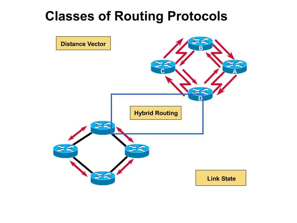
30. The balanced hybrid approach combines aspects of the link-state and distance-vector algorithms. These are really distance-vector routing protocols which apply some of the advantages of a link-state routing protocols, and also known as advanced-distance-vector routing protocols. EIGRP is known as balanced hybrid routing protocol. –EIGRP is covered in CCNP Advanced Routing but it uses many of the concepts from IGRP which we discuss this semester. In the curriculum, IS-IS is described as a balanced hybrid, but it is more often regarded as a link-state routing protocol. –“Examples of hybrid protocols are OSI's IS-IS (Intermediate System-to- Intermediate System), and Cisco's EIGRP (Enhanced Interior Gateway Routing Protocol).” (On-line curriculum)

31. I also disagree with the following information in the on-line curriculum: –“Balanced-hybrid routing protocols use distance vectors with more accurate metrics to determine the best paths to destination networks. However, they differ from most distance-vector protocols by using topology changes to trigger routing database updates.” Balanced hybrid routing protocols don’t necessarily use more accurate metrics than a distance vector routing protocol. EIGRP’s metrics are more accurate than RIP, but not necessarily more accurate than IGRP. RIP and IGRP both use triggered updates during topology changes to speed up network convergence, the same as a balanced hybrid. The real difference is that a hybrid routing protocol like EIGRP does not pass entire routing table information periodically like RIP or IGRP and uses other mechanisms for loop free routing. EIGRP also uses the DUAL algorithm which guarantees loop-free path selection.

32. Topics – (Continued) Part III. Routing Theory and Dynamic Routing Operations (continued) Hybrid Routing Protocols –Concepts –EIGRP (not IS-IS) Path Switching –Example: Host X to Host Y (with three routers in between) –LAN-to-LAN Routing –LAN-to-WAN Routing Cisco Router Configuration Summary Topics (Review)

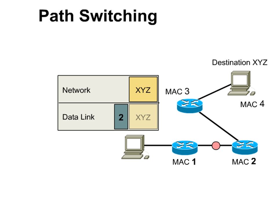
34. Path Switching Host X has a packet(s) to send to Host Y A router generally relays a packet from one data link to another, using two basic functions: 1. a path determination function - Routing 2. a switching function – Packet Forwarding Let’s go through all of the stages these routers use to route and switch this packet. See if you can identify these two functions at each router. Note: Data link addresses have been abbreviated. Path Switching X Y Data Link Header IP (Network layer) Packet Data Link Frame = Data Link Header + IP Packet

35. From Host X to Router RTA Host X begins by encapsulating the IP packet into a data link frame (in this case Ethernet) with RTA’s Ethernet 0 interface’s MAC address as the data link destination address. How does Host X know to forward to packet to RTA and not directly to Host Y? How does Host X know or get RTA’s Ethernet address? –Remember, it looks at the packet’s destination ip address does an AND operation and compares it to its own ip address and subnet mask. –It determines if the two ip addresses are on the same subnet or not. –If they are on the same subnet, it looks for the destination MAC address of the packet in its ARP cache. – sending out an ARP request if it is not there. –If they are on different subnets, it looks for the MAC address of the default gateway in its ARP cache – sending out an ARP request if it is not there. 00-10 0A-10192.168.4.10 192.168.1.10

36. RTA to RTB 1. RTA looks up the IP destination address in its routing table. 192.168.4.0/24 has next-hop-ip address of 192.168.2.2 and an exit- interface of e1. Since the exit interface is on an Ethernet network, RTA must resolve the next-hop-ip address with a destination MAC address. 2. RTA looks up the next-hop-ip address of 192.168.2.2 in its ARP cache. If the entry was not in the ARP cache, the RTA would need to send an ARP request out e1. RTB would send back an ARP reply, so RTA can update its ARP cache with an entry for 192.168.2.2. 0B-31 00-20192.168.4.10 192.168.1.10 1 2 3

37. RTA to RTB (continued) 3. Data link destination address and frame encapsulation After finding the entry for the next-hop-ip address 192.168.2.2 in its ARP cache, RTA uses the MAC address for the destination MAC address in the re-encapsulated Ethernet frame. The frame is now forwarded out Ethernet 1 (as specified in RTA’s routing table. Notice, that the IP Addresses did not change. Also notice that the Routing table was used to find the next-hop ip address, used for the data link address and exit interface, to forward the packet in a new data link frame. 0B-31 00-20192.168.4.10 192.168.1.10 1 2 3

38. FFFF192.168.4.10 192.168.1.10 1 RTB to RTC 1. RTB looks up the IP destination address in its routing table. 192.168.4.0/24 has next-hop-ip address of 192.168.3.2 and an exit- interface of s0 (serial 0). Since the exit interface not on an Ethernet network, RTA does not need to resolve the next-hop-ip address with a destination MAC address. Remember, serial interfaces do not have MAC addresses. 2

39. FFFF192.168.4.10 192.168.1.10 1 RTB to RTC 2. Data link destination address and frame encapsulation. When the interface is a point-to-point serial connection, the Routing Table process does not even look at the next-hop IP address. Remember, a serial link is like a pipe - only one way in and only one way out. RTA now encapsulates the IP packet into the proper data link frame, using the proper serial encapsulation (HDLC, PPP, etc.). The data link destination address is set to a broadcast, since there is only one other end of the pipe and the frame is now forwarded out serial 0. 2

40. 0B-20 0C-22192.168.4.10 192.168.1.10 RTC to Host Y 1. RTC looks up the IP destination address in its routing table. 192.168.4.0/24 is a directly connected network with an exit-interface of e0. RTC realizes that this destination ip address is on the same network as one of its interfaces and it can sent the packet directly to the destination and not another router. Since the exit interface is on an directly connected Ethernet network, RTC must resolve the destination ip address with a destination MAC address. 2. RTC looks up the destination ip address of 192.168.4.10 in its ARP cache. If the entry was not in the ARP cache, the RTC would need to send an ARP request out e0. Host Y would send back an ARP reply, so RTC can update its ARP cache with an entry for 192.168.4.10. 1 3 2

41. 0B-20 0C-22192.168.4.10 192.168.1.10 RTC to Host Y (continued) 3. Data link destination address and frame encapsulation After finding the entry for the destination ip address 192.168.4.10 in its ARP cache, RTC uses the MAC address for the destination MAC address in the re-encapsulated Ethernet frame. The frame is now forwarded out Ethernet 0 (as specified in RTA’s routing table. 1 3 2

42. From Cisco on-line curriculum: When the router checks its routing table entries, it discovers that the best path to destination Network 2 uses outgoing port To0, the interface to a token-ring LAN. Although the lower-layer framing must change as the router passes packet traffic from Ethernet on Network 1 to token-ring on Network 2, the Layer 3 addressing for source and destination remains the same. In the Figure, the destination address remains Network 2, Host 5, regardless of the different lower-layer encapsulations.

43. From Cisco on-line curriculum: Routers enable LAN-to-WAN packet flow by keeping the end-to-end source and destination addresses constant while encapsulating the packet in data link frames, as appropriate, for the next hop along the path. NOTE: Remember, when the interface is a point-to-point serial connection, the Routing Table process does not even look at the next-hop IP address in the routing table, only the exit-interface.

44. Topics – (Continued) Part II. Routing Theory and Dynamic Routing Operations (continued) Hybrid Routing Protocols –Concepts –EIGRP (not IS-IS) Path Switching –Example: Host X to Host Y (with three routers in between) –LAN-to-LAN Routing –LAN-to-WAN Routing Cisco Router Configuration Summary Topics (Review)

45. Topics – (Continued) Part II. Routing Theory and Dynamic Routing Operations (continued) Hybrid Routing Protocols –Concepts –EIGRP (not IS-IS) Path Switching –Example: Host X to Host Y (with three routers in between) –LAN-to-LAN Routing –LAN-to-WAN Routing Cisco Router Configuration Summary Topics (Review)

46. Summary We have covered a lot of topics and a lot of new concepts. These topics will be reinforced when we discuss the specific routing protocols Understanding these concepts is necessary to understand to be able to design, implement, and troubleshoot networks. As we will see, anyone can type in a few commands to enable routing on a router, but if you do not understand these concepts we discussed at best you may not be optimally routing packets in your network and at worst you may be creating routing loops, blackholes, and unreachable networks. Understanding these concepts will also better prepare you for the CCNP Advanced Routing class. Even if you do not take the CCNP Advanced Routing class, these concepts will help you general understanding networking and routing protocols.

47. Cabrillo College Ch. 11 – Routing Basics – End of Part 3 CCNA Semester 2 Rick Graziani, Instructor