1. Compression and Analysis of Very Large Imagery Data Sets Using Spatial Statistics James A. Shine George Mason University and US Army Topographic Engineering Center Interface 2001 June 16, 2001

2. ACKNOWLEDGMENTS §Dr. Margaret Oliver, University of Reading, UK §Dr. Richard Webster, Rothamsted Laboratory, UK §Dr. Daniel Carr, George Mason University

3. INTRODUCTION §Greater resolution in imagery data sets: l pixel resolution (1 meter; 3 x 10^6 data points/square mile) l more bands (up to 256 in hyperspectral sensors;+10^2) l more imagery over time §Compression becomes an important part of timely analysis. §How far can image be compressed before information is lost?

4. PROFESSIONAL MOTIVATION : Collecting imagery, climatic and other topographic data Transforming the data into maps, surfaces, and other topographic products Determination of sampling intervals using spatial statistics is an important tool for many of our applications: collecting ground truth choosing training points for classification

5. DATA SETS

6. CAMIS Data Collection §Computerized Airborne Multicamera Imaging System §Four-band sensor flown in Lear jet (blue, green, red, near infrared) §Each data frame 768x576 pixels §Each flight line has 30 frames §Each collect uses 10-15 flight lines §Order of 10^7 data points per collect

7. Data Preprocessing §Considerable overlap in flight lines §Bands registered to each other first §Overlap removed, forming mosaic §Radiometric correction §Map registration

8. Ft. Story, VA Ft. A.P. Hill, VA

9. SPATIAL STATISTICS Much spatial data (such as imagery) is spatially correlated; points close together have lower variance than those farther apart. Variance can be divided into background noise (stochastic) and spatial. The variance can be modeled by plotting vs. distance between points (variogram) and used for many applications.

10. STOCHASTIC AND SPATIAL VARIATION §STOCHASTIC VARIATION IS LOCAL, BACKGROUND NOISE (NUGGET EFFECT) §SPATIAL VARIATION IS GLOBAL (SILL AND RANGE) §THE SCALE OF SPATIAL VARIATION IS ESPECIALLY IMPORTANT §VARIOGRAMS DEMONSTRATE THESE TWO VARIATIONS

11. HOW TO COMPUTE A VARIOGRAM We have sample locations x1, x2, … and values z at each location. The semivariance for a given distance h is: Where n(h) is the number of pairs of points a distance h apart. The semivariance is then plotted against h as shown on the next slide.

12. MODELING THE VARIOGRAM §The variogram is then fit on several different models: l exponential, nested exponential l spherical, nested spherical l circular l others §The best-fitting model (minimum squared error or a similar metric) is chosen. §The model is then used to determine the scale (or scales in nested models) of variation and for interpolation and estimation.

13. COMPARISON EXPERIMENT §Compute variogram of complete image band §Compute variograms of subsampled image band (reduced by powers of 2) §Compare the variograms, determine when curve is lost §Use this as a compression threshold

14. COMPUTING A FULL IMAGE VARIOGRAM §Data transferred from imagery to text file (ERDAS Imagine, Arc/Info) §Modified FORTRAN program §Running time: approx. 1 hour per 4 x 10^6 points §only 2 directions (N-S and E-W) §Current algorithm O(n^2), may be reducible §Details: Shine, JSM 2000

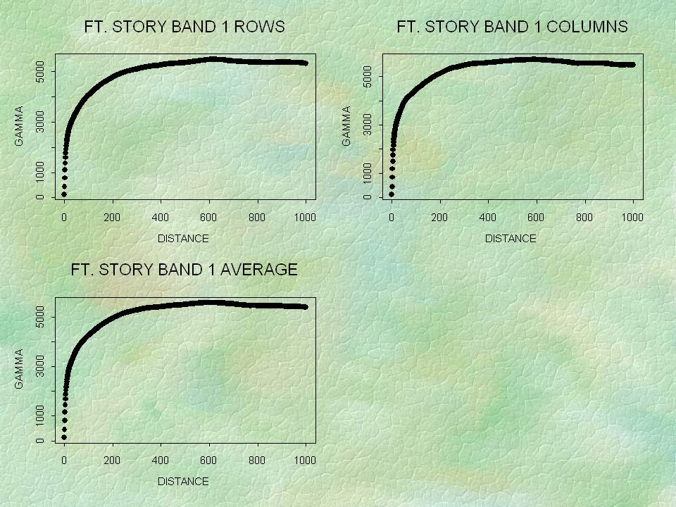
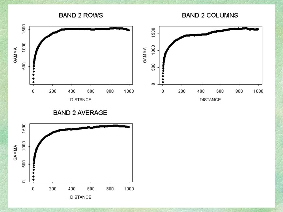
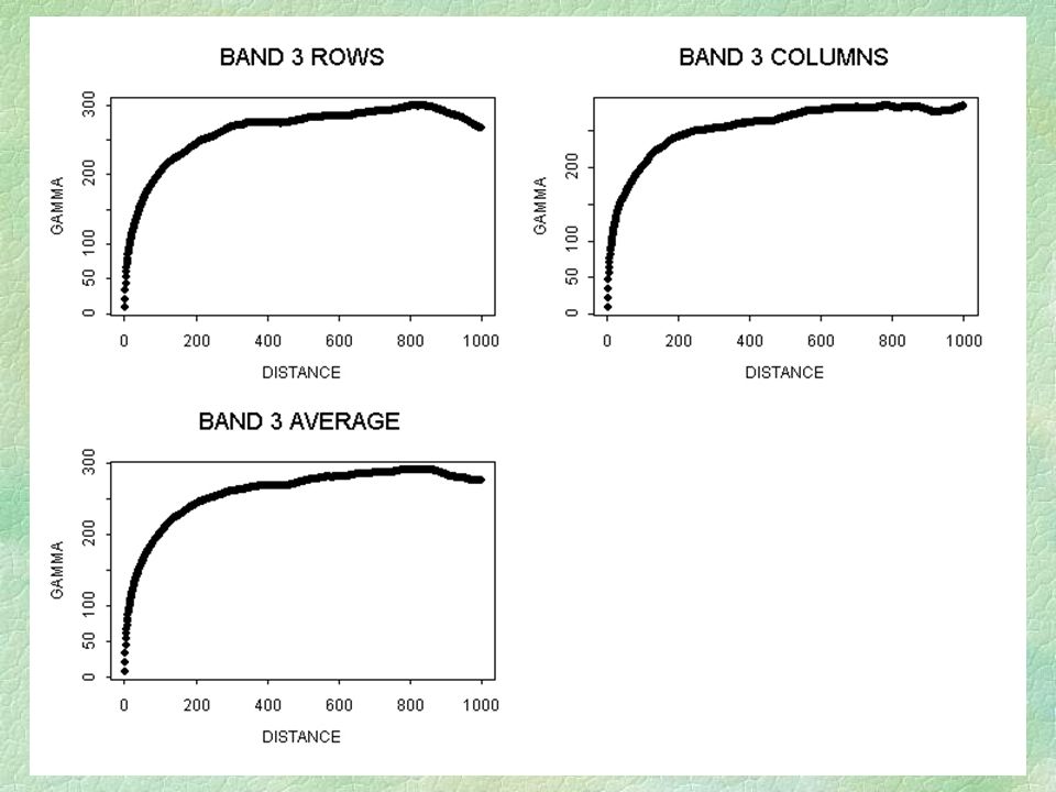
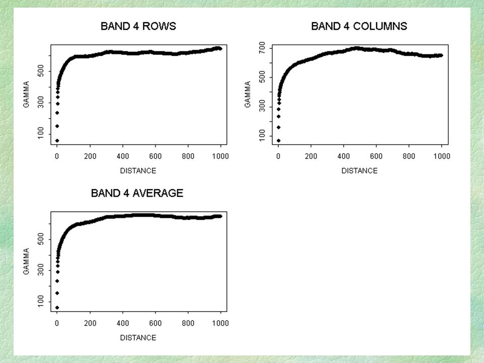
15. Ft. Story full image variograms

19. THEORETICAL VARIOGRAM MODELS

20. A NESTED VARIOGRAM MODEL

21. Ft. A.P. Hill full image variograms

22. BAND 1

26. COMPRESSION ANALYSIS Start with full variogram Reduce sample by ¼ successively Compare resulting variograms

27. EXAMPLE RESULT: A.P. HILL, BAND 1

28. FULL

29. ADD 1/4

30. ADD 1/16

31. ADD 1/64

32. ADD 1/256

33. FULL (ORANGE) AND 1/256 (BLUE) IMAGES SUPERIMPOSED

34. CONCLUSIONS §Preliminary results show little degradation in variogram at 256 times reduction §Seems to indicate that image can be compressed ~10^2 without affecting results of spatial statistical analysis §Computing time savings: hours to minutes

35. FUTURE WORK Optimize variogram code Finish tests on other Ft.A.P. Hill and Ft. Story imagery bands Compare other available CAMIS imagery Obtain general rule for achievable compression for obtaining a spatial correlation model from 1-meter imagery Perform other image analysis operations on original and compressed images and compare.