1. 2.3Logical Implication: Rules of Inference From the notion of a valid argument, we begin a formal study of what we shall mean by an argument and when such an argument is valid. Consider the implication (p 1  p 2  p 3  …  p n )→q. The statements p 1, p 2, p 3, …, p n are called the premises( 前提） of the argument, and the statement q is the conclusion for the argument.

2. 推論證明

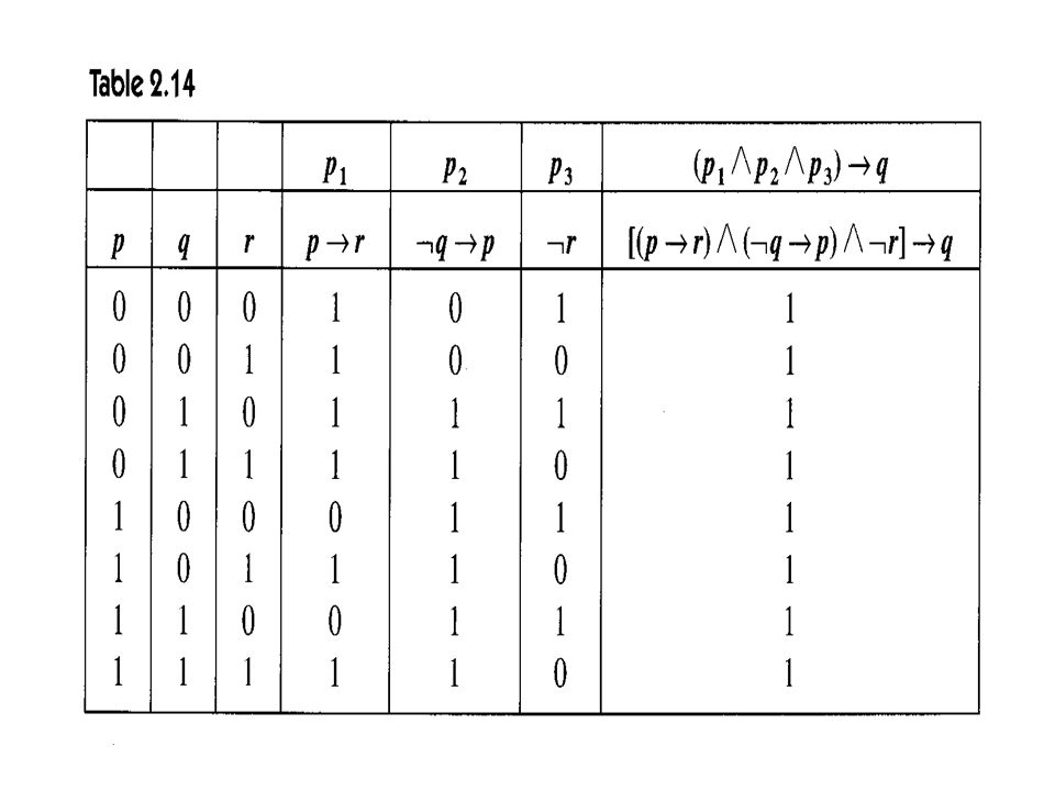
3. Example 2.19: page 69.

5. Example 2.20: page 70. (we know that (p1  p2)→q is a valid argument, and we may say that the truth of the conclusion q is deduced or inferred from the truth of the premises p1, p2.)

6. Definition 2.4: If p, q are arbitrary statements such that p→q is a tautology, then we say that p logically implies q and we write p  q to denote this situation. Note: 1) if p  q, we have p  q and q  p. 2) if p  q and q  p, then we have p  q. 3) p ≠> q is used to indicate that p→q is not a tautology – so the given implication (namely, p→q) is not a logical implication. (See the paragraphs from the bottom of page 70 to the top of page 71.)

7. Example 2.21: page 71.

8. To prove the correctness of a statement, a great deal of the effort must put into constructing the truth tables. And since we want to avoid even larger tables, we are persuaded to develop a list of techniques called rules of inference that help us. (See the top paragraph of page 72.)

9. Example 2.22: page 72. (the Rule of Detachment)

10. Example 2.23: page 73. (the Law of the Syllogism)

11. Example 2.24: page 74.

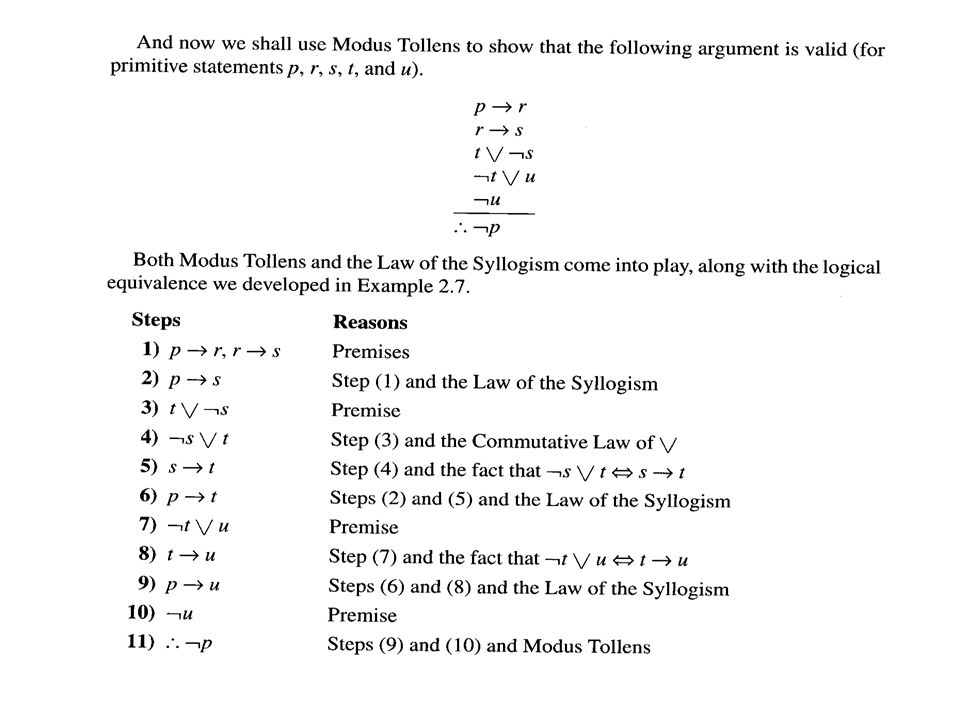
12. Example 2.25: page 75. (Modus Tollens: method of denying)

14. Example 2.26: page 76~77. (the Rule of Conjunction)

15. Example 2.27: page 77

16. Example 2.28: page 77~78. (the Rule of Contradiction)

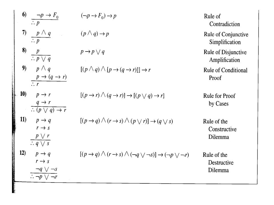
17. Table 2.19: page 79. (Rules of Inference)

19. Example 2.29: page 80

21. Example 2.30

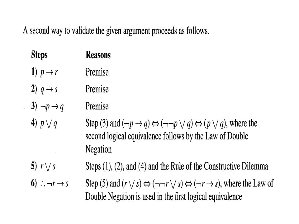
23. Example 2.31: page 81~82.

25. Example 2.32:page 82 反證法

26. (p  (q  r))  ((p^q)  r)

27. Note: [(p1  p2  p3  …  pn) → (q→r)]  [(p1  p2  p3  …  pn  q)→r]. (page 83)

28. Example 2.33: page 84.

30. 2.4The Use of Quantifiers

31. Open statement Sentences that involve a variable, such as x, need not be statements. For example, the sentence "The number x + 2 is an even integer" is not necessarily true or false unless we know what value is substituted for x. If we restrict our choices to integers, then when x is replaced by ‑ 5, ‑ 1, or 3, for instance, the resulting statement is false. In fact, it is false whenever x is replaced by an odd integer. When an even integer is substituted for x, however, the resulting statement is true. We refer to the sentence "The number x + 2 is an even integer" as an open statement, which we formally define as follows.

32. Definition 2.5: A declarative sentence is an open statement if –it contains one or more variables, and –it is not a statement, but –it becomes a statement when the variables in it are replaced by certain allowable choices.

33. Example: “The number x + 2 is an even integer” is an open statement and is denoted by p(x). The allowable choices for x is called the universe (set) for p(x). If x = 3, p(3) is a false statement.

34. Example: “q(x,y): The numbers y + 2, x – y, and x + 2y are even integers.”, then q(4,2) is true. From the above examples, we can say for some x, p(x) (TRUE), for some x, y, q(x,y) (TRUE), or for all x, p(x) (FALSE).

35. Quantifiers Two types of quantifiers, which are called the existential and the universal quantifiers, can quantify the open statements p(x) and q(x,y). the existential quantifier (means “for some x”, “for at least one x”, or “there exists an x such that”): “for some x, p(x)” is denoted as “  x, p(x)”. the universal quantifier (means “for all x”, “for any x”, “for each x”, or “for every x”): “for all x, all y” is denoted by “  x  y”.

36. Example 2.36: page 91.

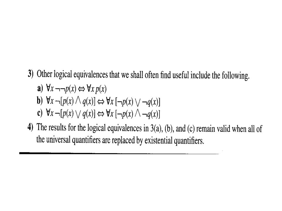
37. Note:  x p(x)   x p(x), but  x p(x) does not logically imply  x p(x).

38. Example 2.38: page 93 (the truth value of a quantified statement may depend on the universe prescribed).

39. Example 2.39: page 94.

40. Table 2.21 summarize and extend some results for quantifiers.

41. Definition 2.6: Let p(x), q(x) be open statements defined for a given universe. The open statements p(x) and q(x) are called (logically) equivalent, and we write  x [p(x)  q(x)] when the biconditional p(a)  q(a) is true for each replacement a from the universe (that is, p(a)  q(a) for each a in the universe). If the implication p(a)  q(a) is true for each a in the universe (that is, p(a)  q(a) for each a in the universe), then we write  x [p(x)  q(x)] and say that p(x) logically implies q(x).

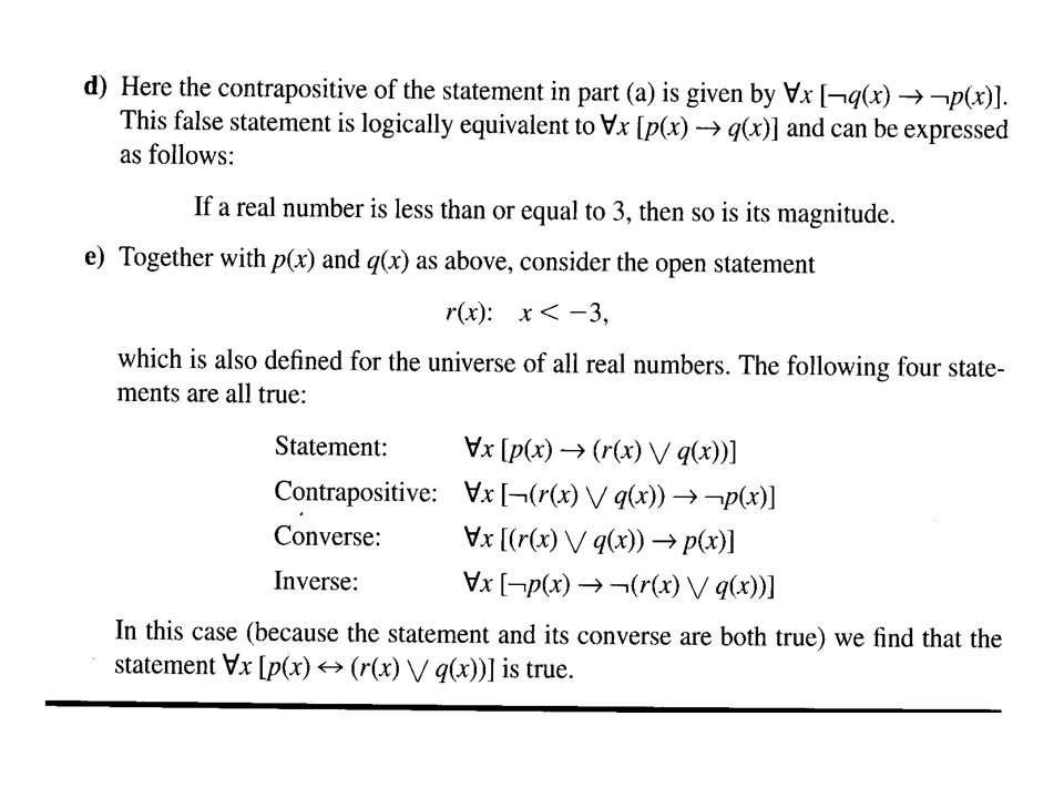
42. Definition 2.7: For open statements p(x), q(x) – defined for a prescribed universe – and the universally quantified statement  x [p(x)  q(x)] we define: –The contrapositive of  x [p(x)  q(x)] to be  x [  q(x)   p(x)]. –The converse of  x [p(x)  q(x)] to be  x [q(x)  p(x)]. –The inverse of  x [p(x)  q(x)] to be  x [  p(x)   q(x)].

43. Example 2.40: page 95~96.

44. Example 2.41: page 96~97.

46. Example 2.42: page 97

47. (the existential quantifier  x does not distribute over the logical connective  ).

48. Table 2.22: Logical equivalences and logical implications for quantified statements in one variable.

49. Example 2.43: page 98.

51. Table 2.23: Rules for negating statements with one quantifier.

52. Example 2.45: page 100.

53. Example 2.46: page 101.

54. Example 2.47: page 101.

55. Example 2.48: page 101

56. 2.5Quantifiers, Definitions, and the Proofs of Theorems In this section we shall combine some of the ideas we have already studied in the prior two sections. The Rule of Universal Specification: If an open statement becomes true for all replacements by the members in a given universe, then that open statement is true for each specific individual member in that universe. (A bit more symbolically – if p(x) is an open statement for a given universe, and if  x p(x) is true, then p(a) is true for each a in the universe.)

57. Example 2.53: page 111.

58. The Rule of Universal Generalization: If an open statement p(x) is proved to be true when x is replaced by any arbitrarily chosen element c from our universe, then the universally quantified statement  x p(x) is true. Furthermore, the rule extends beyond a single variable. So if, for example, we have an open statement q(x,y) that is proved to be true when x and y are replaced by arbitrarily chosen elements from the same universe, or their own respective universes, then the universally quantified statement  x  y q(x, y) [or,  x, y q(x, y)] is true. Similar results hold for the cases of three or more variables.

59. Example 2.54: page 115.

60. Example 2.55: page 116.

61. Example 2.56: page 116~117.

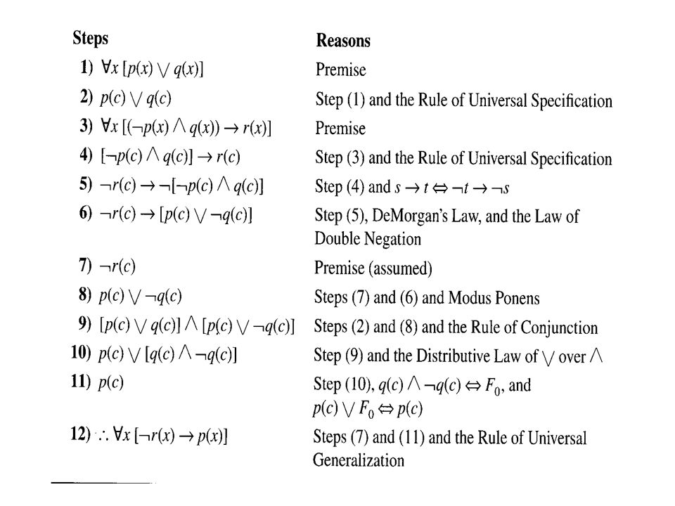
63. The results of Example 2.54 and especially Example 2.56 lead us to believe that we can use universally quantified statements and the rules of inference – including the Rules of Universally Specification and Universal Generalization – to formalize and prove a variety of arguments and, hopefully, theorems.

64. Example:

65. Definition 2.8,

66. Example 2.57

67. Theorem 2.3

68. Theorem 2.4

69. Theorem 2.5