1. Visual FAQ’s on Real Options Celebrating the Fifth Anniversary of the Website: Real Options Approach to Petroleum Investments http://www.puc-rio.br/marco.ind/ By: Marco Antônio Guimarães Dias Petrobras and PUC-Rio, Brazil Real Options 2000 Conference Capitalizing on Uncertainty and Volatility in the New Millennium September 25, 2000  Chicago

2. Visual FAQ’s on Real Options u Selection of frequently asked questions (FAQ’s) by practitioners and academics l Something comprehensive but I confess some bias in petroleum questions l Use of some facilities to visual answer u Real options models present two results: l The value of the investment oportunity (option value) ç How much to pay (or sell) for an asset with options? l The decision rule (thresholds) ç Invest now? Wait and See? Abandon? Expand the production? Switch use of an asset? u Option value and thresholds are the focus of most visual FAQ’s

3. Visual FAQ’s on Real Options: 1 u Are the real options premium important? Real Option Premium = Real Option Value  NPV è Answer with an analogy: l Investments can be viewed as call options ç You get an operating project V (like a stock) by paying the investment cost I (exercise price) ç Sometimes this option has a time of expiration (petroleum, patents, etc.), sometimes is perpetual (real estate, etc.) ç Suppose a 3 years to expiration petroleum undeveloped reserve. The immediate exercise of the option gets the NPV NPV = V  I

4. Real Options Premium u The options premium can be important or not, depending of the of the project moneyness

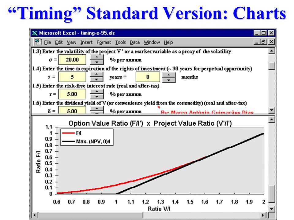
5. Visual FAQ’s on Real Options: 2 u What are the effects of interest rate, volatility, and other parameters in both option value and the decision rule? è Answer with “Timing Suite” l Three spreadsheets that uses a simple model analogy of real options problem with American call option l Lets go to the Excel spreadsheets to see the effects

6. Timing Suite: Real Options Spreadsheets u A set of interactive Excel spreadsheets Timing Suite are used to calculate both the option value and the threshold u Solve American options with the analytic approximation of Barone-Adesi & Whaley (instantaneous response) u The underlying asset is the project value V which can be developed by investing I u Uncertainty: Geometric Brownian Motion, the same of Black-Scholes u Three spreadsheets: l Timing (Standard) l Timing With Two Uncertainties l Timing Switch (two uncertainties)

7. “Timing”: Standard Version

8. “Timing” Standard Version: Charts

10. Timing Suite: Others Spreadsheets u Timing with Two Uncertainties: l Project value V and investment I are both stochastic ç Used again Barone-Adesi & Whaley but for v = V/I. ç This is possible thanks to the PDE first degree homogeneity in V and I: F(V, I, t) = I. F/I(V/I, 1, t) = D. f(v, 1, t) u Timing Switch: abandon and switch use decisions l Myers & Majd (1990) model, case of two risk assets: both project and alternative asset values are uncertain l Exs.: (a) abandon a project for the salvage value; (b) redevelopment of a real estate; (c) conversion of a tanker to a floating production system (oilfield). Exploits analogy with American put and u se the call- put symmetry: C (V, I, r, , T,  ) = P ( I, V,  r, T,  ) ç Knowing the call value you have also the put value & vice versa

11. Visual FAQ’s on Real Options: 3 u Where the real options value comes from? u Why real options value is different of the static net present value (NPV)? è Answer with example: option to expand l Suppose a manager embed an option to expand into her project, by a cost of US$ 1 million The static NPV =  5 million if the option is exercise today, and in future is expected the same negative NPV l Spending a million $ for an expected negative NPV: Is the manager becoming crazy?

12. Uncertainty Over the Expansion Value  Considering combined uncertainties: in product prices and demand, exercise price of the real option, operational costs, etc., the future value (2 years ahead) of the expansion has an expected value of $  5 million l The traditional discount cash will not recommend to embed an option to expansion which is expected to be negative l But the expansion is an option, not an obligation!

13. Option to Expand the Production u Rational managers will not exercise the option to expand @ t = 2 years in case of bad news (negative value) l Option will be exercised only if the NPV > 0. So, the unfavorable scenarios will be pruned (for NPV < 0, value = 0) l Options asymmetry leverage prospect valuation. Option = + 5

14. Real Options Asymmetry and Valuation + = Prospect Valuation Traditional Value =  5 Options Value(T) = + 5 u The visual equation for “Where the options value comes from?”

15. E&P Process and Options u Drill the wildcat? Wait? Extend? u Revelation, option-game: waiting incentives Oil/Gas Success Probability = p Expected Volume of Reserves = B Revised Volume = B’ u Appraisal phase: delineation of reserves u Technical uncertainty: sequential options u Developed Reserves. u Expand the production? u Stop Temporally? Abandon? u Delineated but Undeveloped Reserves. u Develop? “Wait and See” for better conditions? Extend the option?

16. Option to Expand the Production u Analyzing a large ultra-deepwater project in Campos Basin, Brazil, we faced two problems: l Remaining technical uncertainty of reservoirs is still important. In this specific case, the better way to solve the uncertainty is by looking the production profile instead drilling additional appraisal wells l In the preliminary development plan, some wells presented both reservoir risk and small NPV. ç Some wells with small positive NPV (not “deep-in-the- money”) and others even with negative NPV ç Depending of the initial production information, some wells can be not necessary u Solution: leave these wells as optional wells l Small investment to permit a fast and low cost future integration of these wells, depending of both market (oil prices, costs) and the production profile response

17. Modeling the Option to Expand u Define the quantity of wells “deep-in-the-money” to start the basic investment in development u Define the maximum number of optional wells u Define the timing (or the accumulated production) that the reservoir information will be revealed u Define the scenarios (or distributions) of marginal production of each optional well as function of time. l Consider the depletion if we wait after learn about reservoir u Add market uncertainty (reversion + jumps for oil prices) u Combine uncertainties using Monte Carlo simulation (risk-neutral simulation if possible, next FAQ) u Use optimization method to consider the earlier exercise of the option to drill the wells, and calculate option value l Monte Carlo for American options is a frontier research area l Petrobras-PUC project: Monte Carlo for American options

18. Visual FAQ’s on Real Options: 4 u Does risk-neutral valuation mean that investors are risk-neutral? u What is the difference between real simulation and risk-neutral simulation? è Answers l Risk-neutral valuation (RNV) does not assume investors or firms with risk-neutral preferences l RNV does not use real probabilities. It uses risk neutral probabilities (“martingale measure”) Real simulation: real probabilities, uses real drift  Risk-neutral simulation: the sample paths are risk- adjusted. It uses a risk-neutral drift:  ’ = r 

19. Geometric Brownian Motion Simulation  The real simulation of a GBM uses the real drift . The price at future time t is given by: P t = P 0 exp{ (   )  t +  l By sampling the standard Normal distribution N(0, 1) you get the values forP t l With real drift use a risk-adjusted (to P) discount rate  The risk-neutral simulation of a GBM uses the risk-neutral drift  ’ = r . The price at t is: P t = P 0 exp{ (r   )  t +  l With risk-neutral drift, the correct discount rate is the risk-free interest rate.

20. Risk-Neutral Simulation x Real Simulation u For the underlying asset, you get the same value: Simulating with real drift and discounting with risk- adjusted discount rate  ( where  ) Or simulating with risk-neutral drift (r  ) but discounting with the risk-free interest rate (r) u For an option/derivative, the same is not true: Risk-neutral simulation gives the correct option result (discounting with r) but the real simulation does not gives the correct value (discounting with  ) l Why? Because the risk-adjusted discount rate is “adjusted” to the underlying asset, not to the option u Risk-neutral valuation is based on the absence of arbitrage, portfolio replication (complete market) l Incomplete markets: see next FAQ

21. Visual FAQ’s on Real Options: 5 u Is possible to use real options for incomplete markets? u What change? What are the possible ways? è Answer: Yes, is possible to use. l For incomplete markets the risk-neutral probability (martingale measure) is not unique l So, risk-neutral valuation is not rigorously correct because there is a lack of market values l Academics and practitioners use some ways to estimate the real option value, see next slide

22. Incomplete Markets and Real Options u In case of incomplete market, the alternatives to real options valuation are: l Assume that the market is approximately complete (your estimative of market value is reliable) and use risk-neutral valuation (with risk-neutral probability) l Assume firms are risk-neutral and discount with risk-free interest rate (with real probability) l Specify preferences (the utility function) of single-agent or the equilibrium at detailed level (Duffie) ç Used by finance academics. In practice is difficult to specify the utility of a corporation (managers, stockholders) l Use the dynamic programming framework with an exogenous discount rate ç Used by academics economists: Dixit & Pindyck, Lucas, etc. ç Corporate discount rate express the corporate preferences?

23. Visual FAQ’s on Real Options: 6 u Is true that mean-reversion always reduces the options premium? u What is the effect of jumps in the options premium? è Answers: l First, we’ll see some different processes to model the uncertainty over the oil prices (for example) l Second, we’ll compare the option premium for an oilfield using different stochastic processes ç All cases are at-the-money real options (current NPV = 0) ç The equilibrium price is 20 $/bbl for all reversion cases

24. Geometric Brownian Motion (GBM) u This is the most popular stochastic process, underlying the famous Black-Scholes-Merton options equation l GBM: expected curve is a exponential growth (or decrease); prices have a log-normal distribution in every future time; and the variance grows linearly with the time

25. u In this process, the price tends to revert toward a long- run average price (or an equilibrium level) P. l Model analogy: spring (reversion force is proportional to the distance between current position and the equilibrium level). l In this case, variance initially grows and stabilize afterwards l Charts: the variance of distributions stabilizes after t i Mean-Reverting Process

26. Nominal Prices for Brent and Similar Oils (1970-1999) u We see oil prices jumps in both directions, depending of the kind of abnormal news: jumps-up in 1973/4, 1978/9, 1990, 1999; and jumps-down in 1986, 1991, 1997 Jumps-up Jumps-down

27. Mean-Reversion + Jumps for Oil Prices u Adopted in the Marlim Project Finance (equity modeling) a mean-reverting process with jumps:  The jump size/direction are random:  ~ 2N l In case of jump-up, prices are expected to double  OBS: E(  ) up = ln2 = 0.6931 l In case of jump-down, prices are expected to halve  OBS: ln(½) =  ln2 =  0.6931 where: (the probability of jumps) (jump size)

28. Equation for Mean-Reversion + Jumps u The interpretation of the jump-reversion equation is: mean-reversion drift: positive drift if P < P negative drift if P > P { uncertainty over the continuous process (reversion) { variation of the stochastic variable for time interval dt uncertainty over the discrete process (jumps) continuous (diffusion) process discrete process (jumps)

29. Mean-Reversion x GBM: Option Premium u The chart compares mean-reversion with GBM for an at-the-money project at current 25 $/bbl l NPV is expected to revert from zero to a negative value Reversion in all cases: to 20 $/bbl

30. Mean-Reversion with Jumps x GBM u Chart comparing mean-reversion with jumps versus GBM for an at-the-money project at current 25 $/bbl l NPV still is expected to revert from zero to a negative value

31. Mean-Reversion x GBM u Chart comparing mean-reversion with GBM for an at- the-money project at current 15 $/bbl (suppose) l NPV is expected to revert from zero to a positive value

32. Mean-Reversion with Jumps x GBM u Chart comparing mean-reversion with jumps versus GBM for an at-the-money project at current 15 $/bbl (suppose) l Again NPV is expected to revert from zero to a positive value

33. Visual FAQ’s on Real Options: 7 u How to model the effect of the competitor entry in my investment decisions? è Answer : option-games, the combination of the real options with game-theory l First example: Duopoly under Uncertainty (Dixit & Pindyck, 1994; Smets, 1993) ç Demand for a product follows a GBM ç Only two players in the market for that product (duopoly)

34. Duopoly Entry under Uncertainty u The leader entry threshold: both players are indifferent about to be the leader or the follower. l Entry: NPV > 0 but earlier than monopolistic case

35. Other Example: Oil Drilling Game u Oil exploration: the waiting game of drilling u Two companies X and Y with neighbor tracts and correlated oil prospects: drilling reveal information l If Y drills and the oilfield is discovered, the success probability for X’s prospect increases dramatically. If Y drilling gets a dry hole, this information is also valuable for X. l Here the effect of the competitor presence is the opposite: to increase the value of waiting to invest Company X tract Company Y tract

36. Visual FAQ’s on Real Options: 8 u Does Real Options Theory (ROT) speed up the firms investments or slow down investments? è Answer: depends of the kind of investment l ROT speeds up today strategic investments that create options to invest in the future. Examples: investment in capabilities, training, R&D, exploration, new markets... l ROT slows down large irreversible investment of projects with positive NPV but not “deep in the money” l Large projects but with high profitability (“deep in the money”) must be done by both ROT and static NPV.

37. Visual FAQ’s on Real Options: 9 u Is possible real options theory to recommend investment in a negative NPV project? è Answer: yes, mainly sequential options with investment revealing new informations l Example: exploratory oil prospect (Dias 1997) ç Suppose a “now or never” option to drill a wildcat ç Static NPV is negative and traditional theory recommends to give up the rights on the tract ç Real options will recommend to start the sequential investment, and depending of the information revealed, go ahead (exercise more options) or stop

38. Sequential Options (Dias, 1997)  Traditional method, looking only expected values, undervaluate the prospect (EMV =  5 MM US$): l There are sequential options, not sequential obligations; l There are uncertainties, not a single scenario. ( Wildcat Investment ) ( Developed Reserves Value ) ( Appraisal Investment: 3 wells ) ( Development Investment ) Note: in million US$ “Compact Decision-Tree” EMV =  15 + [20% x (400  50  300)]  EMV =  5 MM$

39. Sequential Options and Uncertainty u Suppose that each appraisal well reveal 2 scenarios (good and bad news) èdevelopment option will not be exercised by rational managers èoption to continue the appraisal phase will not be exercised by rational managers

40. Option to Abandon the Project u Assume it is a “now or never” option u If we get continuous bad news, is better to stop investment u Sequential options turns the EMV to a positive value u The EMV gain is  3.25  5) = $ 8.25 being: (Values in millions) $ 2.25 stopping development $ 6 stopping appraisal $ 8.25 total EMV gain

41. Visual FAQ’s on Real Options: 10 u Is the options decision rule (invest at or above the threshold curve) the policy to get the maximum option value? u How much value I lose if I invest a little above or little below the optimum threshold? è Answer: yes, investing at or above the threshold line you maximize the option value. è But sometimes you don’t lose much investing near of the optimum (instead at the optimum) l Example: oilfield development as American call option. Suppose oil prices follow a GBM to simplify.

42. Thresholds: Optimum and Sub-Optima u The theoretical optimum (red) of an American call option (real option to develop an oilfield) and the sub-optima thresholds (~10% above and below)

43. Optima Region u Using a risk-neutral simulation, I find out here that the optimum is over a “plateau” (optima region) not a “hill” u So, investing ~ 10% above or below the theoretical optimum gets rough the same value

44. Real Options Premium u Now a relation optimum with option premium is clear: near of the point A (theoretical threshold) the option premium can be very small.

45. Visual FAQ’s on Real Options: 11 u How Real Options Sees the Choice of Mutually Exclusive Alternatives to Develop a Project? è Answer: very interesting and important application l Petrobras-PUC is starting a project to compare alternatives of development, alternatives of investment in information, alternatives with option to expand, etc. l One simple model is presented by Dixit (1993). l Let see directly in the website this model

46. Conclusions u The Visual FAQ’s on Real Options illustrated: l Option premium; visual equation for option value; uncertainty modeling; decision rule (thresholds); risk- neutral x real simulation/valuation; Timing Suite; effect of competition; optimum problem, etc. l The idea was to develop the intuition to understand several results in the real options literature l The use of real options changes real assets valuation and decision making when compared with static NPV u There are several other important questions l The Visual FAQ’s on Real Options is a webpage with a growth option! l Don’t miss the new updates with the new FAQ’s at: ç http://www.puc-rio.br/marco.ind/faqs.html