1. Insurance Applications of Bivariate Distributions David L. Homer & David R. Clark CAS Annual Meeting November 2003

2. AGENDA: Explain the Insurance problem being addressed Explain the Insurance problem being addressed Show the mathematical “machinery” used to address the problem Show the mathematical “machinery” used to address the problem Provide a numerical example Provide a numerical example

4. The Players: Insured: Dietrichson Drilling A large account with predictable annual losses Insurer: Pacific All Risk Insurance Co. Actuary:You

5. The Pricing Problem: Pacific All-Risk Insurance Company sells a product that provides coverage on both Specific Excess – individual losses above 600,000 Specific Excess – individual losses above 600,000 Aggregate Excess – above the sum of all retained losses capped at 3,000,000 in the aggregate Aggregate Excess – above the sum of all retained losses capped at 3,000,000 in the aggregate

6. 3,000,0008,000,000 1,000,000 600,000 Aggregate Losses Per-occurrence Retained by the insured Per-Occurrence Layer Stop Loss Layer Policy Structure proposed for our insured Dietrichson Drilling

7. How do we price this product? Expected Losses are straight-forward Expected Losses are straight-forward Expected Losses for the two coverages are additive Expected Losses for the two coverages are additive Separate distributions are straight- forward Separate distributions are straight- forward A combined distribution is NOT A combined distribution is NOT

9. How do we estimate a single distribution? Define frequency and severity distributions, then: Heckman-Meyers Heckman-Meyers Recursive methods (Panjer) Recursive methods (Panjer) Simulation Simulation Fast Fourier Transform (FFT) Fast Fourier Transform (FFT)

10. Key Elements of FFT Technique: Discretized severity vector x=(x 0,…,x n-1 ) Discretized severity vector x=(x 0,…,x n-1 ) FFT formula FFT formula IFFT formula IFFT formula

11. Convolution Theorem: The transform of the sum is equal to the product of the transforms. To sum up j independent identical variables:

12. Probability Generating Function: PGF N The PGF N is a short-cut method for combining the distributions for each possible number of claims. It does all of the convolutions for us!

13. Putting it all together we obtain the aggregate probability vector z from the severity probability vector x and the claim count PGF N :

14. Bivariate case is the same, but using a MATRIX instead of a VECTOR. becomes becomes…

16. Pacific All-Risk: Severity Distribution Bivariate Severity M x 0 0.00% 200,000 37.80% 400,000 23.50% 600,000 14.60% 800,000 9.10% 1,000,000 15.00% Primary ExcessMarginal 0200,000400,000600,000 0 0.00% 0.00% 0.00% 0.00% 0.00% 200,00037.80% 0.00% 0.00% 0.00%37.80% 400,00023.50% 0.00% 0.00% 0.00%23.50% 600,00014.60% 9.10%15.00% 0.00%38.70% 800,000 0.00% 0.00% 0.00% 0.00% 0.00% 1,000,000 0.00% 0.00% 0.00% 0.00% 0.00% Excess Marginal75.90% 9.10%15.00% 0.00%100.00% Primary Single Claim Severity x

17. Negative Binomial PGF for claim counts with Mean=5 and Variance=6:

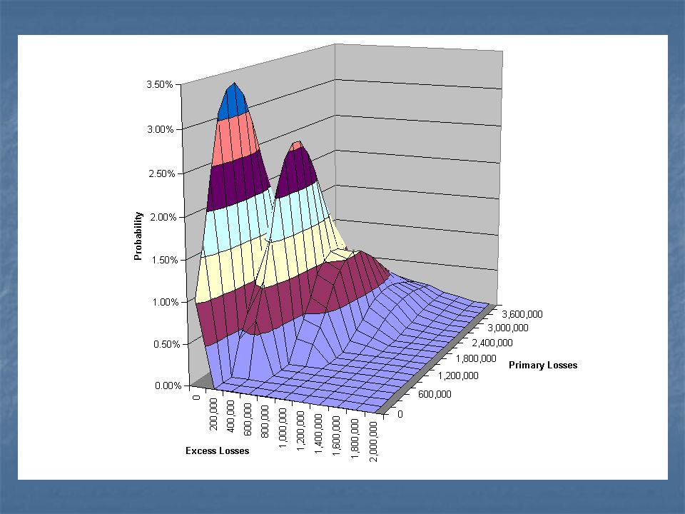
18. Bivariate Aggregate Matrix M z 0200,000400,000600,000800,0001,000,0001,200,000 01.05%0.00%0.00%0.00%0.00%0.00%0.00% 200,0001.65%0.00%0.00%0.00%0.00%0.00%0.00% 400,0002.38%0.00%0.00%0.00%0.00%0.00%0.00% 600,0003.09%0.40%0.66%0.00%0.00%0.00%0.00% 800,0003.34%0.65%1.07%0.00%0.00%0.00%0.00% 1,000,0003.39%0.96%1.58%0.00%0.00%0.00%0.00% 1,200,0003.22%1.27%2.16%0.26%0.21%0.00%0.00% 1,400,0002.86%1.40%2.44%0.44%0.36%0.00%0.00% 1,600,0002.43%1.45%2.59%0.66%0.54%0.00%0.00% 1,800,0001.97%1.40%2.57%0.90%0.78%0.09%0.05% 2,000,0001.54%1.26%2.38%1.02%0.92%0.15%0.08% 2,200,0001.17%1.09%2.12%1.08%1.01%0.24%0.13% 2,400,0000.86%0.90%1.80%1.08%1.05%0.33%0.20% 2,600,0000.62%0.72%1.47%1.00%1.01%0.38%0.24% 2,800,0000.43%0.55%1.16%0.88%0.93%0.42%0.27% 3,000,0000.29%0.41%0.89%0.75%0.82%0.43%0.29% Primary Excess

20. Probability Distribution for Per-Occurrence Excess Losses

21. Expected Per-Occurrence Loss =391,000overall =830,334in scenarios where stop loss is hit Both coverages go bad at the same time!

22. Other Applications: Generation of Large & Small losses for DFA Generation of Large & Small losses for DFA Loss and ALAE with separate limits Loss and ALAE with separate limits Any other bivariate phenomenon Any other bivariate phenomenon (e.g., WC medical and indemnity)

23. Questions or Comments?