Download presentation
Presentation is loading. Please wait.

1
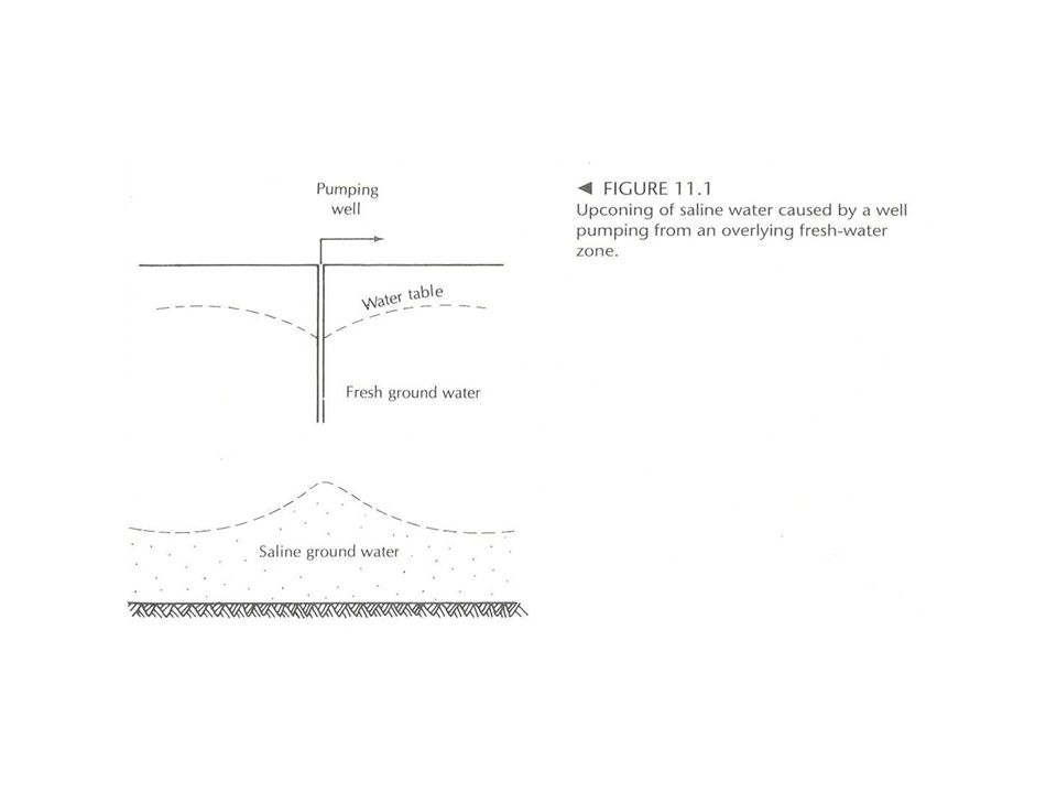
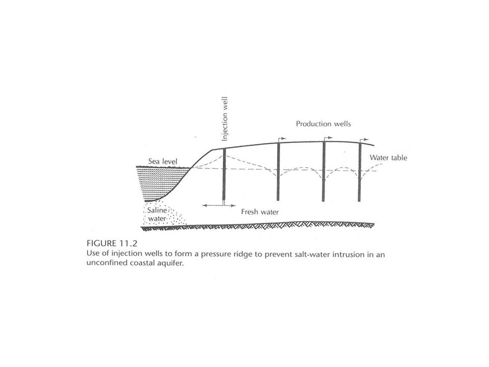
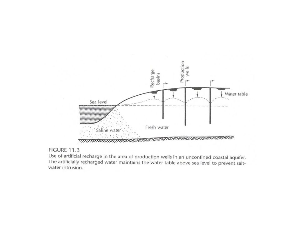
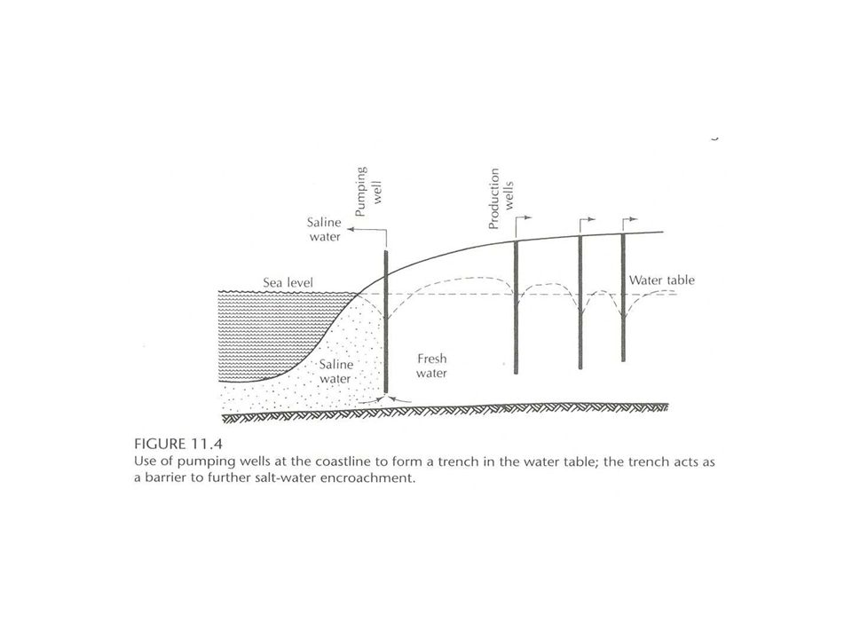
Ground-water flow to wells Extract water Remove contaminated water Lower water table for constructions Relieve pressures under dams Injections – recharges Control slat-water intrusion

2
Our purpose of well studies Compute the decline in the water level, or drawdown, around a pumping well whose hydraulic properties are known. Determine the hydraulic properties of an aquifer by performing an aquifer test in which a well is pumped at a constant rate and either the stabilized drawdown or the change in drawdown over time is measured.

4
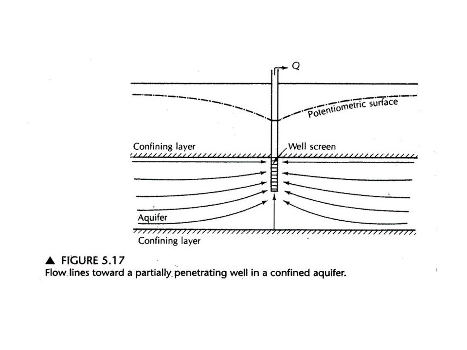
Our Wells Fully penetrate aquifers Radial symmetric Aquifers are homogeneous and isotropic

5
Basic Assumptions The aquifer is bounded on the bottom by a confining layer. All geologic formations are horizontal and have infinite horizontal extent. The potentiometric surface of the aquifer is horizontal prior to the start of the pumping. The potentiometric surface of the aquifer is not recharging with time prior to the start of the pumping. All charges in the position of the potentiometric surface are due to the effect of the pumping alone.

6
Basic Assumptions (cont.) The aquifer is homogeneous and isotropic. All flow is radial toward the well. Ground water flow is horizontal. Darcy’s law is valid. Ground water has a constant density and viscosity. The pumping well and the observation wells are fully penetrating. The pumping well has an infinitesimal diameter and is 100% efficient.

8
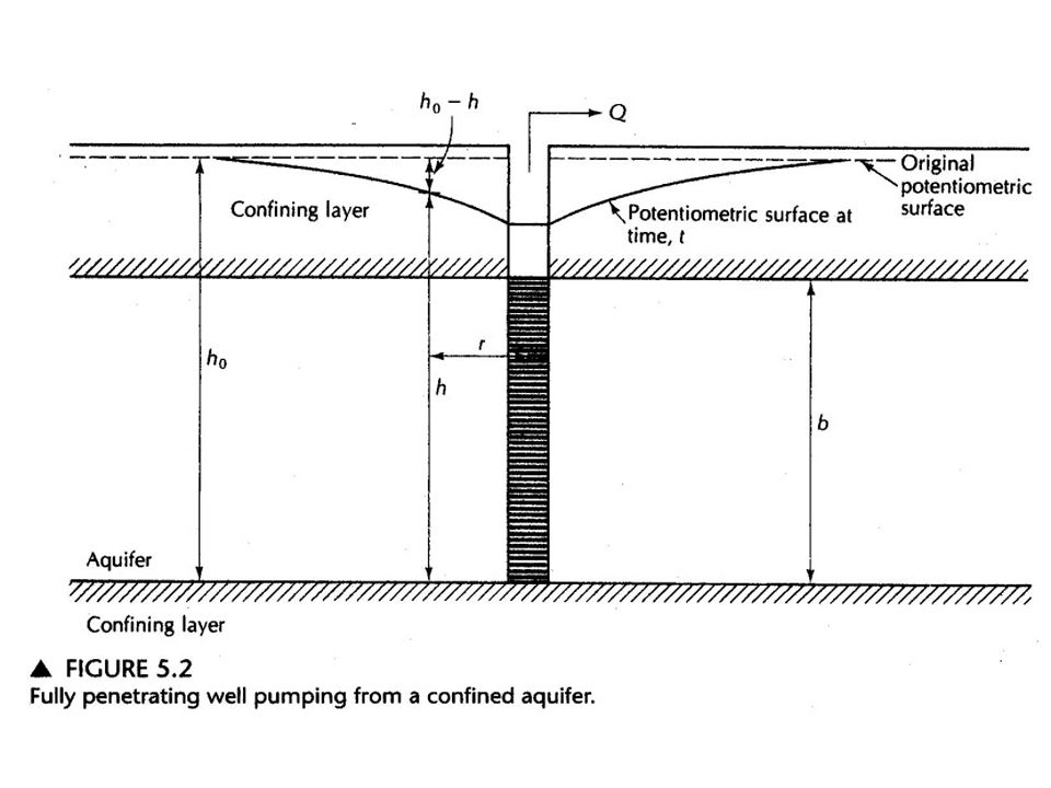
A completely confined aquifer Addition assumptions: The aquifer is confined top and bottom. The is no source of recharge to the aquifer. The aquifer is compressible. Water is released instantaneously. Constant pumping rate of the well.

10
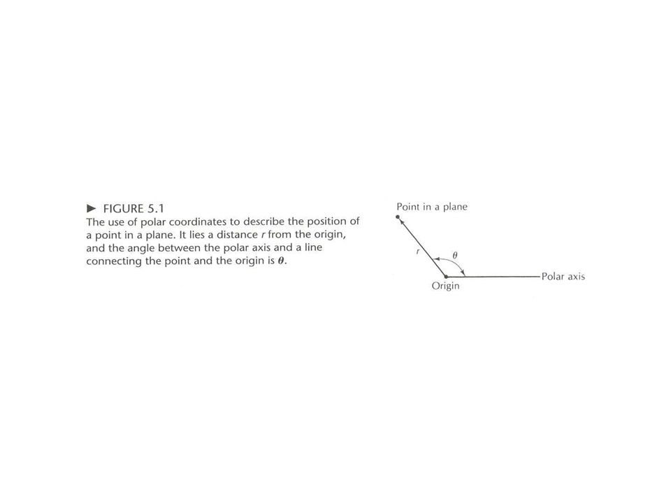
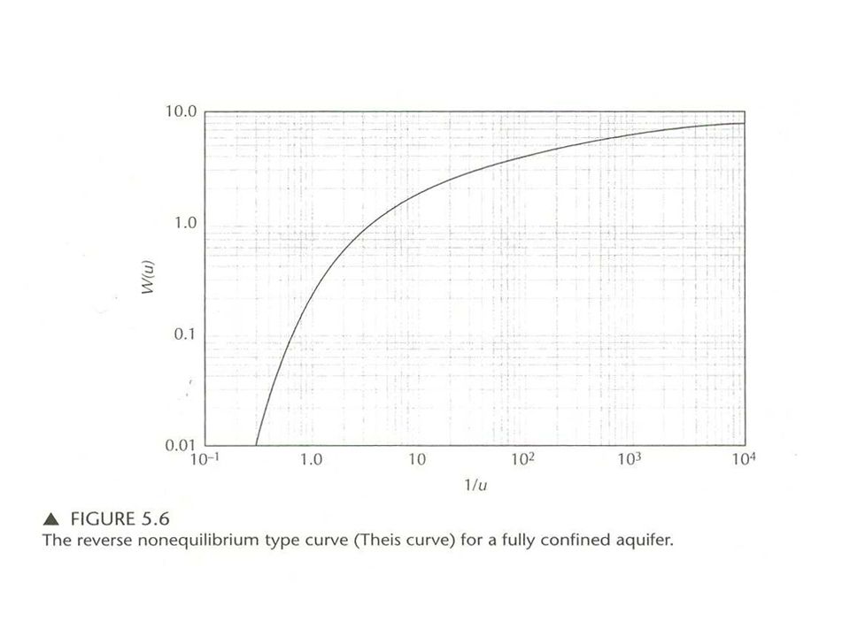
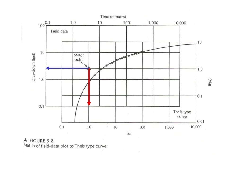
Theis (nonequilibrium) Equation h 0 – h = (Q/4πT) W(u) h 0 = initial hydraulic head (L; m or ft) h = hydraulic head (L; m or ft) h 0 – h = drawdown (L; m or ft) Q = constant pumping rate (L 3 /T; m 3 /d or ft 3 /d) W(u) = well function. T = transmissivity (L 2 /T; m 2 /d or ft 2 /d)
.")
11
Theis (nonequilibrium) Equation u = (r 2 S/4Tt) T = transmissivity (L 2 /T; m 2 /d or ft 2 /d) S = storativity (dimensionless) t = time since pumping began (T; d) r = radial distance from the pumping well (L; m or ft)
 Equation u = (r 2 S/4Tt) T = transmissivity (L 2 /T; m 2 /d or ft 2 /d) S = storativity (dimensionless) t = time since pumping began (T; d) r = radial distance from the pumping well (L; m or ft)")
12
Well Function W(u) = u (e -a /a) da = -0.5772 + ln u + u – u 2 /22! + u 3 /33! – u 4 /44! + …
 = u (e -a /a) da = ln u + u – u 2 /22! + u 3 /33! – u 4 /44! + …")
14
A Leaky, Confined Aquifer Equations

16
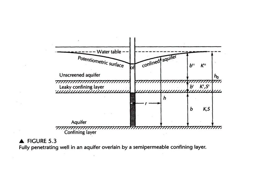
A Leaky, Confined Aquifer – no water drains from the confining layer The aquifer is bounded on the top by an aquitard. The aquitard is overlain by an unconfined aquifer, know as the source bed. The water table in the source bed is initially horizontal. The water table in the source bed does not fall during pumping of the aquifer.

17
A Leaky, Confined Aquifer – no water drains from the confining layer Ground water flow in the aquitard is vertical. The aquifer is compressible, and water drains instantaneously with a decline in head The aquitard is incompressible, so that no water is released from storage in the aquitard when the aquifer is pumped.

18
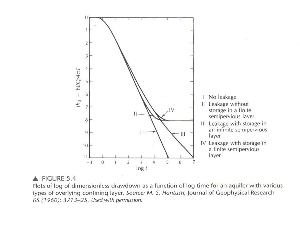
Wells in Confined Aquifers Completely confined aquifer. Confined, leaky with no elastic storage in the leaky layer. Confined, leaky with elastic storage in the leaky layer.

19
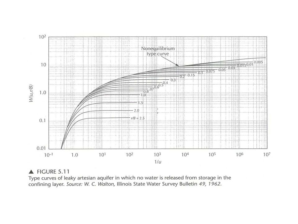
Hantush-Jacob Formula Confined with no elastic storage h 0 – h = (Q/4πT) W(u,r/B) h 0 = initial hydraulic head (L; m or ft) h = hydraulic head (L; m or ft) h 0 – h = drawdown (L; m or ft) Q = constant pumping rate (L 3 /T; m 3 /d or ft 3 /d) W(u,r/B) = leaky artesian well function T = transmissivity (L 2 /T; m 2 /d or ft 2 /d) B = (Tb’/K’) 1/2
 W(u,r/B) h 0 = initial hydraulic head (L; m or ft) h = hydraulic head (L; m or ft) h 0 – h = drawdown (L; m or ft) Q = constant pumping rate (L 3 /T; m 3 /d or ft 3 /d) W(u,r/B) = leaky artesian well function T = transmissivity (L 2 /T; m 2 /d or ft 2 /d) B = (Tb’/K’) 1/2")
21
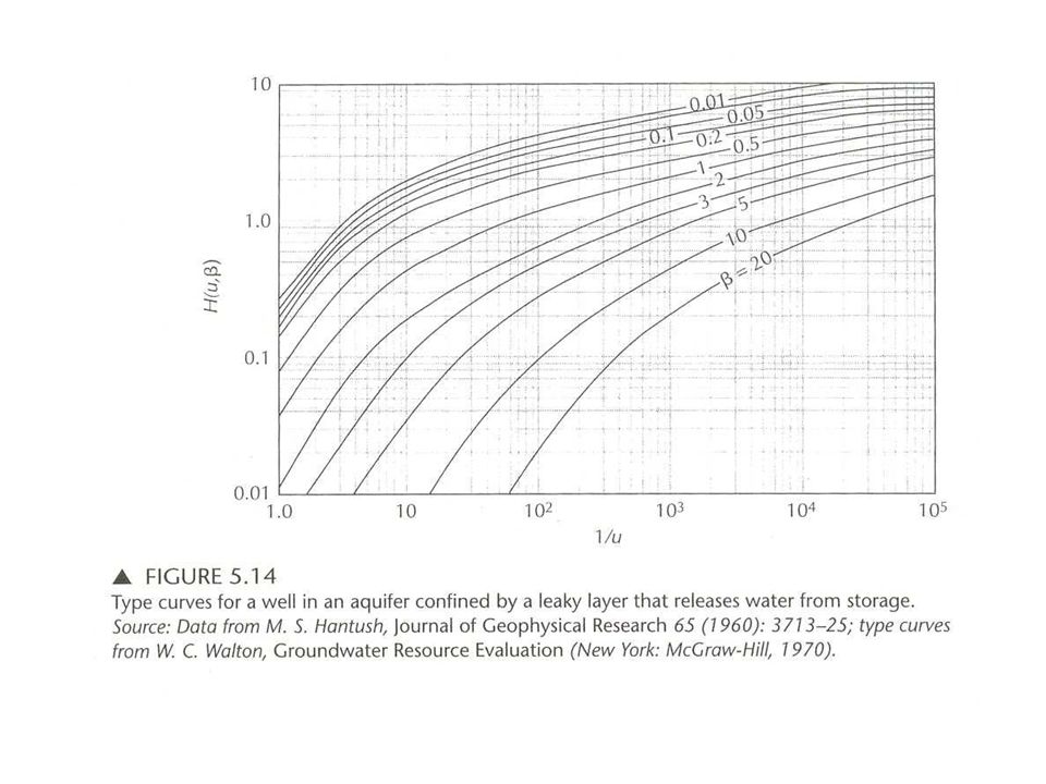
Drawdown Formula Confined with elastic storage h 0 – h = (Q/4πT) H(u, ) h 0 = initial hydraulic head (L; m or ft) h = hydraulic head (L; m or ft) h 0 – h = drawdown (L; m or ft) Q = constant pumping rate (L 3 /T; m 3 /d or ft 3 /d) H(u, ) = a modified leaky artesian well function T = transmissivity (L 2 /T; m 2 /d or ft 2 /d) = r/4B (S’/S) 1/2 ; B = (Tb’/K’) 1/2
 H(u, ) h 0 = initial hydraulic head (L; m or ft) h = hydraulic head (L; m or ft) h 0 – h = drawdown (L; m or ft) Q = constant pumping rate (L 3 /T; m 3 /d or ft 3 /d) H(u, ) = a modified leaky artesian well function T = transmissivity (L 2 /T; m 2 /d or ft 2 /d) = r/4B (S’/S) 1/2 ; B = (Tb’/K’) 1/2")
24
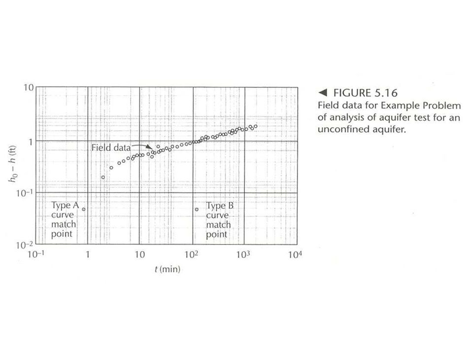
Unconfined aquifer – 3 phases Early stage – pressure drops specific storage as a major contribution behaves as an artesian aquifer flow is horizontal time-drawdown follows Theis curve S - the elastic storativity.

25
Unconfined aquifer – 3 phases Second stage – water table declines specific yield as a major contribution flow is both horizontal and vertical time-drawdown is a function of K v /K h r, b

26
Unconfined aquifer – 3 phases Later stage – rate of drawdown decreases flow is again horizontal time-drawdown again follows Theis curve S - the specific yield.

27
Neuman’ assumptions Aquifer is unconfined. Vadose zone has no influence on the drawdown. Water initially pumped comes from the instantaneous release of water from elastic storage. Eventually water comes from storage due to gravity drainage of interconnected pores.

28
Neuman’ assumptions (cont.) The drawdown is negligible compared to the saturated thickness. The specific yield is at least 10 times the elastic storativity. The aquifer may be – but does not have to be – anisotropic with the radial hydraulic conductivity different than the vertical hydraulic conductivity.

29
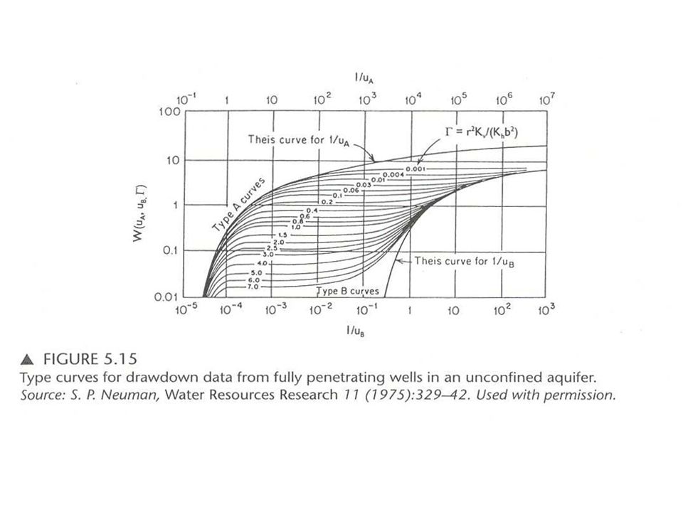
Drawdown Formula unconfined with elastic storage h 0 – h = (Q/4πT) W(u A,u B, ) h 0 = initial hydraulic head (L; m or ft) h = hydraulic head (L; m or ft) h 0 – h = drawdown (L; m or ft) Q = constant pumping rate (L 3 /T; m 3 /d or ft 3 /d) W(u A,u B, ) = the well function for water-table aquifer T = transmissivity (L 2 /T; m 2 /d or ft 2 /d) u A =r 2 S/(4Tt); u B =r 2 Sy/(4Tt); =r 2 Kv/(r 2 Kh)
 W(u A,u B, ) h 0 = initial hydraulic head (L; m or ft) h = hydraulic head (L; m or ft) h 0 – h = drawdown (L; m or ft) Q = constant pumping rate (L 3 /T; m 3 /d or ft 3 /d) W(u A,u B, ) = the well function for water-table aquifer T = transmissivity (L 2 /T; m 2 /d or ft 2 /d) u A =r 2 S/(4Tt); u B =r 2 Sy/(4Tt); =r 2 Kv/(r 2 Kh)")
31
Drawdown T = Q/ 4 (h 0 -h)G(u) G(u) = W(u) - completely confined. W(u,r/B) – leaky, confined, no storage. H(u, ) – leaky, confined, with storage. W(u A,u B, ) - unconfined.
 – leaky, confined, no storage. H(u, ) – leaky, confined, with storage. W(u A,u B, ) - unconfined..")
33
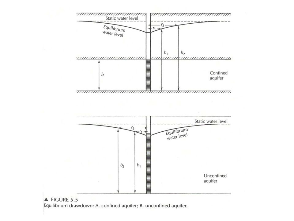
Steady-radial flow in a confined Aquifer The aquifer is confined top and bottom. Well is pumped at a constant rate. Equilibrium has reached.

35
Steady-radial flow in a unconfined Aquifer The aquifer is unconfined and underlain by a horizontal aquiclude. Well is pumped at a constant rate. Equilibrium has reached.

37
Drawdown T = Q/ 4 (h 0 -h)G(u) G(u) = W(u) - completely confined. W(u,r/B) – leaky, confined, no storage. H(u, ) – leaky, confined, with storage. W(u A,u B, ) - unconfined.
 – leaky, confined, no storage. H(u, ) – leaky, confined, with storage. W(u A,u B, ) - unconfined..")
38
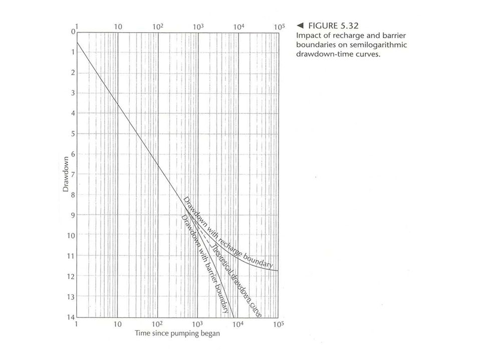
Aquifer test Steady-state conditions. Cone of depression stabilizes. Nonequilibrium flow conditions. Cone of depression changes. Needs a pumping well and at least one observational well.

39
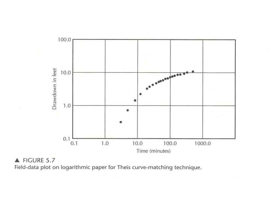
Transient flow in a confined Aquifer – Theis Method

43
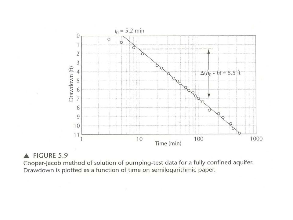
Transient flow in a confined aquifer – Cooper-Jacob Method T = 2.3Q/4 (h 0 -h) log (2.25Tt/(r 2 S)). Only valid when u, (r 2 S/4Tt) < 0.05 --- after some time of pumping
 < after some time of pumping.")
45
Transient flow in a confined aquifer – Cooper-Jacob Method T = 2.3Q/ 4 (h 0 -h) S = 2.25Tt 0 /r 2 (h 0 -h) – drawdown per log cycle of time t 0 - is the time, where the straight line intersects the zero-drawdown axis.
 S = 2.25Tt 0 /r 2 (h 0 -h) – drawdown per log cycle of time t 0 - is the time, where the straight line intersects the zero-drawdown axis.")
47
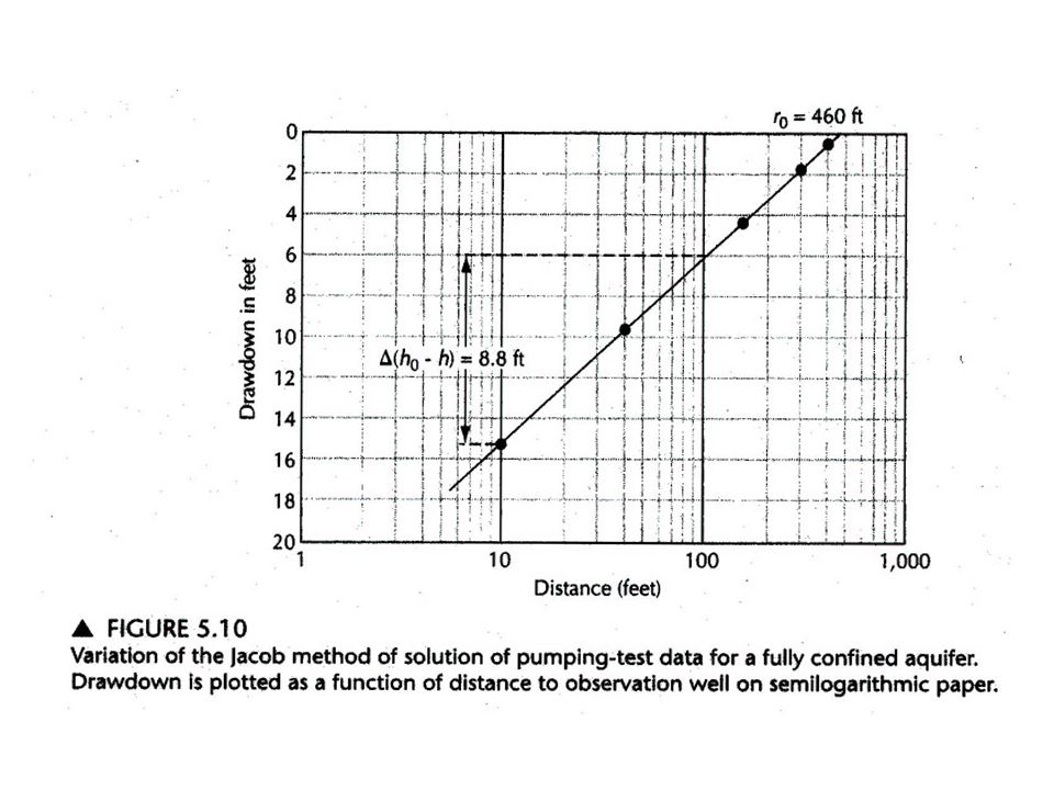
Transient flow in a confined aquifer – Cooper-Jacob Method T = 2.3Q/ 2 (h 0 -h) S = 2.25Tt/r 0 2 (h 0 -h) – drawdown per log cycle of distance r 0 - is the distance, where the straight line intersects the zero-drawdown axis.
 S = 2.25Tt/r 0 2 (h 0 -h) – drawdown per log cycle of distance r 0 - is the distance, where the straight line intersects the zero-drawdown axis.")
48
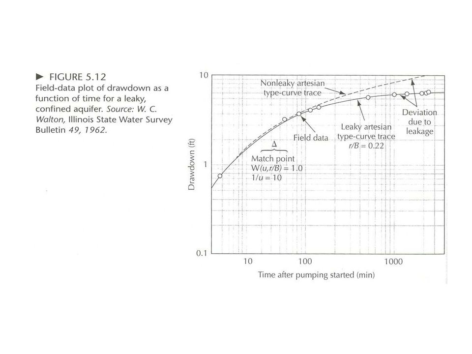
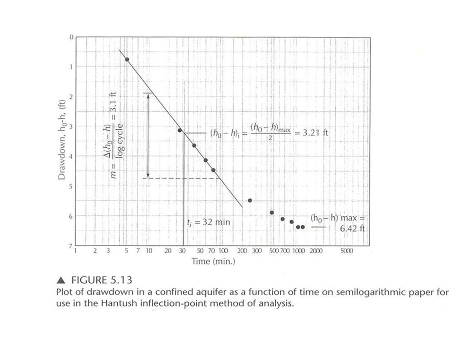
Transient flow in a leaky, confined aquifer with no storage. Walton Graphic method Hantush inflection-point method.

49
Transient flow in a leaky, confined aquifer with no storage T = Q/ 4 (h 0 -h)W(u,r/B) S = 4Tut/r 2 r/B = r /(Tb’/K’) 1/2 K’ = [Tb’(r/B) 2 ]/r 2
![Transient flow in a leaky, confined aquifer with no storage T = Q/ 4 (h 0 -h)W(u,r/B) S = 4Tut/r 2 r/B = r /(Tb’/K’) 1/2 K’ = [Tb’(r/B) 2 ]/r 2](http://images.slideplayer.com/25/8069954/slides/slide_49.jpg "Transient flow in a leaky, confined aquifer with no storage T = Q/ 4 (h 0 -h)W(u,r/B) S = 4Tut/r 2 r/B = r /(Tb’/K’) 1/2 K’ = [Tb’(r/B) 2 ]/r 2")
53
Transient flow in a leaky, confined aquifer with storage T = Q/ 4 (h 0 -h)H(u, ) S = 4Tut/r 2 2 = r 2 S’ / (16 B 2 S) B = (Tb’/K’) 1/2 K’S’ = [16 2 Tb’S]/r 2
![Transient flow in a leaky, confined aquifer with storage T = Q/ 4 (h 0 -h)H(u, ) S = 4Tut/r 2 2 = r 2 S’ / (16 B 2 S) B = (Tb’/K’) 1/2 K’S’ = [16 2 Tb’S]/r 2](http://images.slideplayer.com/25/8069954/slides/slide_53.jpg "Transient flow in a leaky, confined aquifer with storage T = Q/ 4 (h 0 -h)H(u, ) S = 4Tut/r 2 2 = r 2 S’ / (16 B 2 S) B = (Tb’/K’) 1/2 K’S’ = [16 2 Tb’S]/r 2")
55
Transient flow in an unconfined aquifer T = Q/ 4 (h 0 -h)W(u A,u B, ) S = 4Tu A t/r 2 (for early drawdown) S y = 4Tu B t/r 2 (for later drawdown) = r 2 K v /b 2 K h
W(u A,u B, ) S = 4Tu A t/r 2 (for early drawdown) S y = 4Tu B t/r 2 (for later drawdown) = r 2 K v /b 2 K h")
58
Aquifer tests T = Q/ 4 (h 0 -h)G(u) G(u) = W(u) - completely confined. W(u,r/B) – leaky, confined, no storage. H(u, ) – leaky, confined, with storage. W(u A,u B, ) - unconfined.
 – leaky, confined, no storage. H(u, ) – leaky, confined, with storage. W(u A,u B, ) - unconfined..")
60
Aquifer tests T = Q/ 4 (h 0 -h)G(u) G(u) = W(u) - completely confined. W(u,r/B) – leaky, confined, no storage. H(u, ) – leaky, confined, with storage. W(u A,u B, ) - unconfined.
 – leaky, confined, no storage. H(u, ) – leaky, confined, with storage. W(u A,u B, ) - unconfined..")
64
Transient flow in a confined aquifer – Cooper-Jacob Method T = 2.3Q/4 (h 0 -h) log (2.25Tt/(r 2 S)). Only valid when u, (r 2 S/4Tt) < 0.05 --- after some time of pumping
 < after some time of pumping.")
66
Transient flow in a confined aquifer – Cooper-Jacob Method T = 2.3Q/ 4 (h 0 -h) S = 2.25Tt 0 /r 2 (h 0 -h) – drawdown per log cycle of time t 0 - is the time, where the straight line intersects the zero-drawdown axis.
 S = 2.25Tt 0 /r 2 (h 0 -h) – drawdown per log cycle of time t 0 - is the time, where the straight line intersects the zero-drawdown axis.")
68
Transient flow in a confined aquifer – Cooper-Jacob Method T = 2.3Q/ 2 (h 0 -h) S = 2.25Tt/r 0 2 (h 0 -h) – drawdown per log cycle of distance r 0 - is the distance, where the straight line intersects the zero-drawdown axis.
 S = 2.25Tt/r 0 2 (h 0 -h) – drawdown per log cycle of distance r 0 - is the distance, where the straight line intersects the zero-drawdown axis.")
69
Aquifer test Steady-state conditions. Cone of depression stabilizes. Nonequilibrium flow conditions. Cone of depression changes. Needs a pumping well and at least one observational well.

71
Steady-radial flow in a confined Aquifer The aquifer is confined top and bottom. Well is pumped at a constant rate. Equilibrium has reached.

73
Steady-radial flow in a unconfined Aquifer The aquifer is unconfined and underlain by a horizontal aquiclude. Well is pumped at a constant rate. Equilibrium has reached.

75
Our purpose of well studies Compute the decline in the water level, or drawdown, around a pumping well whose hydraulic properties are known. Determine the hydraulic properties of an aquifer by performing an aquifer test in which a well is pumped at a constant rate and either the stabilized drawdown or the change in drawdown over time is measured.

76
Drawdown T = Q/ 4 (h 0 -h)G(u) G(u) = W(u) - completely confined. W(u,r/B) – leaky, confined, no storage. H(u, ) – leaky, confined, with storage. W(u A,u B, ) - unconfined.
 – leaky, confined, no storage. H(u, ) – leaky, confined, with storage. W(u A,u B, ) - unconfined..")
77
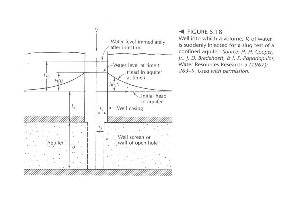
Slug test Goal – to determine the hydraulic conductivity of the formation in the immediate vicinity of a monitoring well. Means – A known volume of water is quickly drawn from or added to the monitoring, the rate which the water level rises or falls is measured and analyzed.

78
Slug test Overdamped – water level recovers to the initial static level in a smooth manner that is approximately exponential. Underdamped – water level oscillates about the static water level with the magnitude of oscillation decreasing with time until the oscillations cease.

80
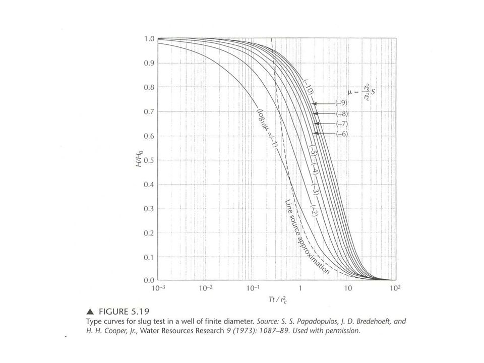
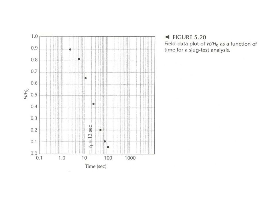
Cooper-Bredehoeft-Papadopulos Method (confined aquifer) H/H 0 = F( , ) H – head at time t. H 0 – head at time t = 0. = T t/r c 2 = r s 2 S/r c 2

83
Cooper-Bredehoeft-Papadopulos Method (confined aquifer) H/H 0 = 1, = 1 at match point. = T t 1 /r c 2 = r s 2 S/r c 2

84
Underdamped Response Slug Test

85
Van der Kamp Method – confined aquifer and well fully penetrating. H(t) = H 0 e - t cos t H(t) - hydraulic head (L) at time t (T) H 0 - the instantaneous change in head (L) - damping constant (T -1 ) - an angular frequency (T -1 )
 = H 0 e - t cos t H(t) - hydraulic head (L) at time t (T) H 0 - the instantaneous change in head (L) - damping constant (T -1 ) - an angular frequency (T -1 ).")
86
Underdamped Response Slug Test (cont.) T = c + a ln T c = -a ln[0.79 r s 2 S(g/L) 1/2 ] a = [r c 2 (g/L) 1/2 ] / (8d) d = /(g/L) 1/2 L = g / ( 2 + 2 )
![Underdamped Response Slug Test (cont.) T = c + a ln T c = -a ln[0.79 r s 2 S(g/L) 1/2 ] a = [r c 2 (g/L) 1/2 ] / (8d) d = /(g/L) 1/2 L = g / ( 2 + 2 )](http://images.slideplayer.com/25/8069954/slides/slide_86.jpg "Underdamped Response Slug Test (cont.) T = c + a ln T c = -a ln[0.79 r s 2 S(g/L) 1/2 ] a = [r c 2 (g/L) 1/2 ] / (8d) d = /(g/L) 1/2 L = g / ( 2 + 2 )")
87
= ln[H(t 1 )/H(t 2 )]/ (t 2 – t 1 ) = 2 /(t 2 -t 1 )
![ = ln[H(t 1 )/H(t 2 )]/ (t 2 – t 1 ) = 2 /(t 2 -t 1 )](http://images.slideplayer.com/25/8069954/slides/slide_87.jpg " = ln[H(t 1 )/H(t 2 )]/ (t 2 – t 1 ) = 2 /(t 2 -t 1 )")
88
Underdamped Response Slug Test (cont.) T 1 = c + a ln c T 2 = c + a ln T 1 Till, L computed from L = g / ( 2 + 2 ) With 20% of the value as computed by L = L c + (r c 2 /r s 2 )(b/2)
 T 1 = c + a ln c T 2 = c + a ln T 1 Till, L computed from L = g / ( 2 + 2 ) With 20% of the value as computed by L = L c + (r c 2 /r s 2 )(b/2)")
89
Aquifer tests T = Q/ 4 (h 0 -h)G(u) G(u) = W(u) - completely confined. W(u,r/B) – leaky, confined, no storage. H(u, ) – leaky, confined, with storage. W(u A,u B, ) - unconfined.
 – leaky, confined, no storage. H(u, ) – leaky, confined, with storage. W(u A,u B, ) - unconfined..")
90
Slug test Overdamped – water level recovers to the initial static level in a smooth manner that is approximately exponential. Underdamped – water level oscillates about the static water level with the magnitude of oscillation decreasing with time until the oscillations cease.

98
x = -y/tan(2 Kbiy/Q) Q - pumping rate K - conductivity b – initial thickness i – initial h gradient x 0 = -Q/tan(2 Kbi) y max = Q/(2Kbi) Confined
 Q - pumping rate K - conductivity b – initial thickness i – initial h gradient x 0 = -Q/tan(2 Kbi) y max = Q/(2Kbi) Confined")
99
Capture Zone Analysis (unconfined aquifer) x = -y / tan[ K[h 1 2 -h 2 2 )y/QL] x 0 = -QL/[ K(h 1 2 -h 2 2 )] y max = QL/[K (h 1 2 -h 2 2 )]
![Capture Zone Analysis (unconfined aquifer) x = -y / tan[ K[h 1 2 -h 2 2 )y/QL] x 0 = -QL/[ K(h 1 2 -h 2 2 )] y max = QL/[K (h 1 2 -h 2 2 )]](http://images.slideplayer.com/25/8069954/slides/slide_99.jpg "Capture Zone Analysis (unconfined aquifer) x = -y / tan[ K[h 1 2 -h 2 2 )y/QL] x 0 = -QL/[ K(h 1 2 -h 2 2 )] y max = QL/[K (h 1 2 -h 2 2 )]")
100
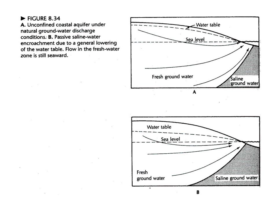
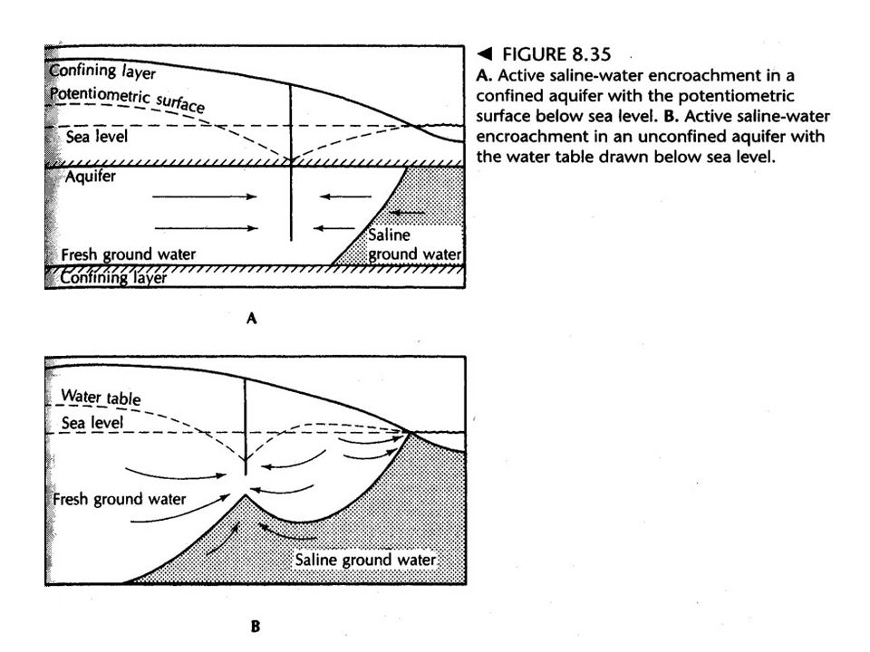
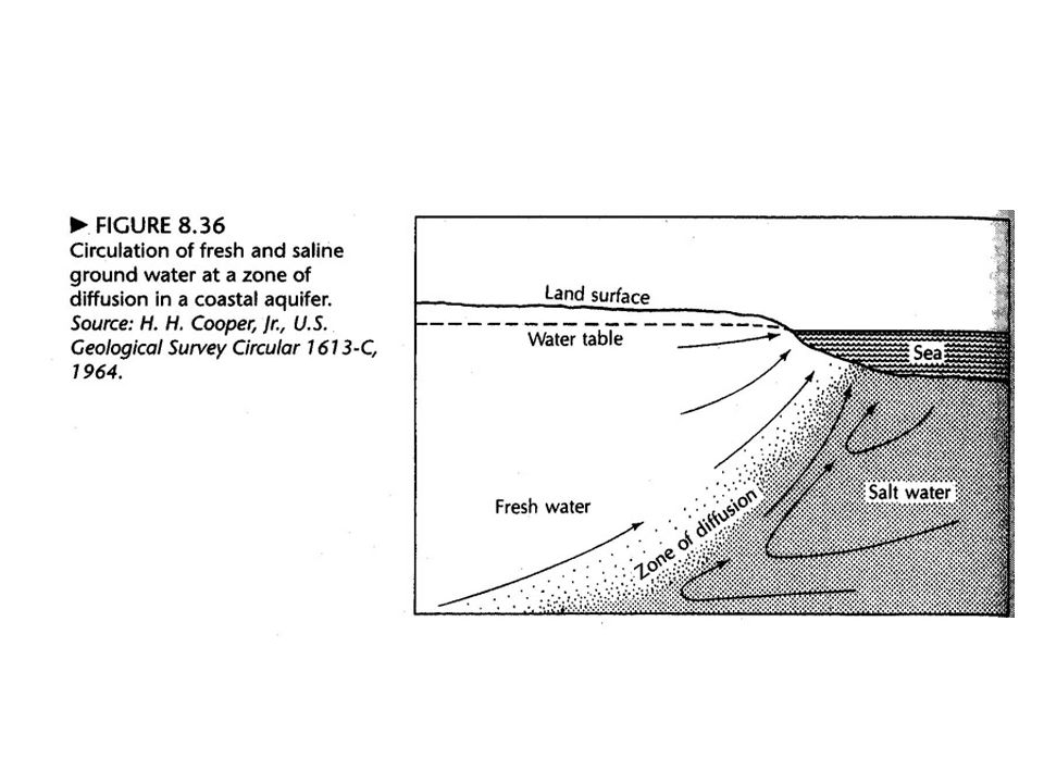
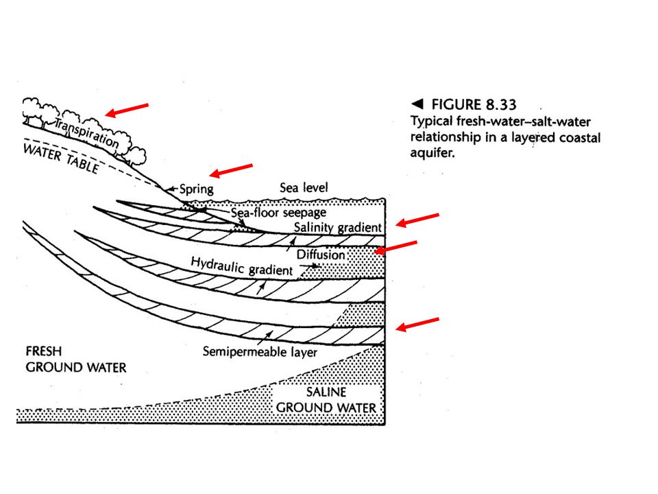
Static fresh and slat water Ghyben-Herzberg principle

104
Dupuit assumptions Hydraulic gradient is equal to the slope of the water table. For small water-table gradients, the streamlines are horizontal and equipotential lines are vertical.

105
z = [2Gq’x/K] 1/2 Dupit-Ghyben-Herzberg model
![z = [2Gq’x/K] 1/2 Dupit-Ghyben-Herzberg model](http://images.slideplayer.com/25/8069954/slides/slide_105.jpg "z = [2Gq’x/K] 1/2 Dupit-Ghyben-Herzberg model")
106
z = [G 2 q’ 2 /K 2 + 2Gq’x/K] 1/2 x 0 = - Gq’/2K
![z = [G 2 q’ 2 /K 2 + 2Gq’x/K] 1/2 x 0 = - Gq’/2K](http://images.slideplayer.com/25/8069954/slides/slide_106.jpg "z = [G 2 q’ 2 /K 2 + 2Gq’x/K] 1/2 x 0 = - Gq’/2K")
107
H x = H 0 exp[-x( S/t 0 T) 1/2 ] t T = x(t 0 S/4 T) 1/2 t 0 tide period
![H x = H 0 exp[-x( S/t 0 T) 1/2 ] t T = x(t 0 S/4 T) 1/2 t 0 tide period](http://images.slideplayer.com/25/8069954/slides/slide_107.jpg "H x = H 0 exp[-x( S/t 0 T) 1/2 ] t T = x(t 0 S/4 T) 1/2 t 0 tide period")
115
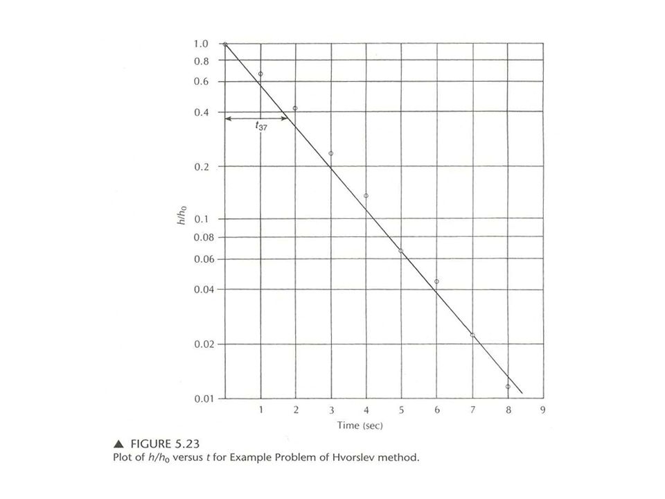
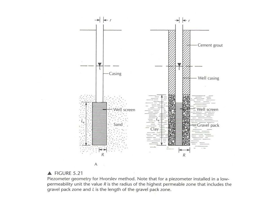
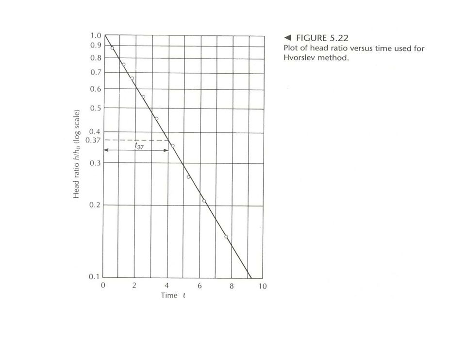
Hvorslev Method (partially penetrated well) Log (h/h 0 ) ~ time t (L e /R > 8) h – head at time t; h 0 – head at time t = 0. K = (r 2 ln (L e /R))/(2L e t 37 ) K – hydraulic conductivity (L/T; ft/d, m/d); r – radius of the well casing (L; ft, m); R – radius of well screen (L; ft, m); L e – length of the well screen (L; ft, m); t 37 – time it takes for water level to rise or fall to 37% of the initial change, (T; d, s).
)/(2L e t 37 ) K – hydraulic conductivity (L/T; ft/d, m/d); r – radius of the well casing (L; ft, m); R – radius of well screen (L; ft, m); L e – length of the well screen (L; ft, m); t 37 – time it takes for water level to rise or fall to 37% of the initial change, (T; d, s)..")
118
Hvorslev Method (partially penetrated well) Log (h/h 0 ) ~ time t (L e /R > 8) h – head at time t; h 0 – head at time t = 0. K = (r 2 ln (L e /R))/(2L e t 37 ) K – hydraulic conductivity (L/T; ft/d, m/d); r – radius of the well casing (L; ft, m); R – radius of well screen (L; ft, m); L e – length of the well screen (L; ft, m); t 37 – time it takes for water level to rise or fall to 37% of the initial change, (T; d, s).
)/(2L e t 37 ) K – hydraulic conductivity (L/T; ft/d, m/d); r – radius of the well casing (L; ft, m); R – radius of well screen (L; ft, m); L e – length of the well screen (L; ft, m); t 37 – time it takes for water level to rise or fall to 37% of the initial change, (T; d, s)..")
119
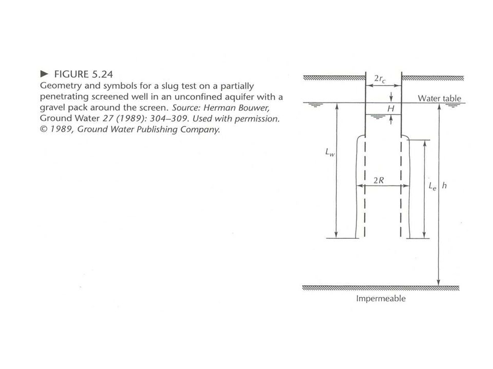
Bouwer and Rice Method K = r c 2 ln (R e /R)/2L e 1/t ln(H 0 /H t ) K – hydraulic conductivity (L/T; ft/d, m/d); r – radius of the well casing (L; ft, m); R – radius of gravel envelope (L; ft, m); R e – effective radial distance over which head is dissipated (L; ft, m); L e – length of the well screen (L; ft, m); t – time since H = H 0 H – head at time t; H 0 – head at time t = 0.
/2L e 1/t ln(H 0 /H t ) K – hydraulic conductivity (L/T; ft/d, m/d); r – radius of the well casing (L; ft, m); R – radius of gravel envelope (L; ft, m); R e – effective radial distance over which head is dissipated (L; ft, m); L e – length of the well screen (L; ft, m); t – time since H = H 0 H – head at time t; H 0 – head at time t = 0.")
120
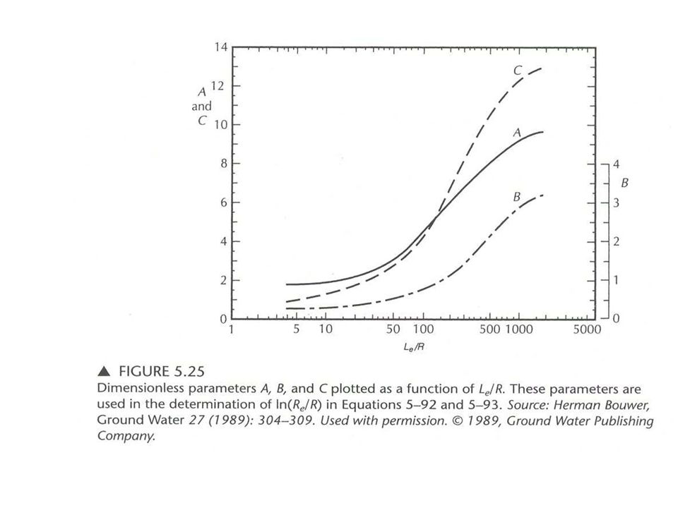
Bouwer and Rice Method ln (R e /R) = [1.1/ln(L w /R) + (A+B ln(h- L w )/R)/(L e /R)] -1 (L w < h) ln (R e /R) = [1.1/ln(L w /R) + C/(L e /R)] -1 (L w = h)
![Bouwer and Rice Method ln (R e /R) = [1.1/ln(L w /R) + (A+B ln(h- L w )/R)/(L e /R)] -1 (L w < h) ln (R e /R) = [1.1/ln(L w /R) + C/(L e /R)] -1 (L w = h)](http://images.slideplayer.com/25/8069954/slides/slide_120.jpg "Bouwer and Rice Method ln (R e /R) = [1.1/ln(L w /R) + (A+B ln(h- L w )/R)/(L e /R)] -1 (L w < h) ln (R e /R) = [1.1/ln(L w /R) + C/(L e /R)] -1 (L w = h)")
123
(1/t) ln(H 0 /H t ) = [1/(t 2 -t 1 )]ln(H 1 /H 2 ) t1t1 t2t2 H1H1 H2H2
![(1/t) ln(H 0 /H t ) = [1/(t 2 -t 1 )]ln(H 1 /H 2 ) t1t1 t2t2 H1H1 H2H2](http://images.slideplayer.com/25/8069954/slides/slide_123.jpg "(1/t) ln(H 0 /H t ) = [1/(t 2 -t 1 )]ln(H 1 /H 2 ) t1t1 t2t2 H1H1 H2H2")
124
This reflects K of The undisturbed aquifer

125
Transmissivity from specific capacity data Specific capacity = yield/drawdown. T = Q/(h 0 -h) 2.3/4 log (2.25Tt/(r 2 S)). T = 15.3 [Q/(h 0 -h)] 0.67 [m,d] T = 33.6 [Q/(h 0 -h)] 0.67 [ft,d] T = 0.76 [Q/(h 0 -h)] 1.08 [m,d]
 2.3/4 log (2.25Tt/(r 2 S)). T = 15.3 [Q/(h 0 -h)] 0.67 [m,d] T = 33.6 [Q/(h 0 -h)] 0.67 [ft,d] T = 0.76 [Q/(h 0 -h)] 1.08 [m,d].")
Similar presentations


>")


>")


