1. Financial Risk Management of Insurance Enterprises Financial Scenario Generators

2. Financial Scenario Project Optional Discussion Session Tuesday, March 11 8-10 pm 162 Education

3. Modeling of Economic Series Research Sponsored by the Casualty Actuarial Society and the Society of Actuaries Investigators: Kevin Ahlgrim, ASA, PhD, Illinois State University Steve D’Arcy, FCAS, PhD, University of Illinois Rick Gorvett, FCAS, ARM, FRM, PhD, University of Illinois

4. Outline of Presentation Motivation for Financial Scenario Generator Project Short description of included economic variables An overview of the model Applications of the model Comparison of this model with another actuarial return generating model Conclusions

5. ERM Frameworks: “Traditional” Risk Management Process 1.Identify loss exposure 2.Measure impact potential 3.Evaluate alternative methods of control 4.Implement best alternative 5.Monitor outcomes

6. COSO ERM Framework

7. ERM Frameworks: “Traditional” Risk Management Process 1.Identify loss exposure 2.Measure impact potential 3.Evaluate alternative methods of control –Based on “risk appetite” of organization 4.Implement best alternative 5.Monitor outcomes

8. Overview of Project CAS/SOA Request for Proposals on “Modeling of Economic Series Coordinated with Interest Rate Scenarios” –A key aspect of dynamic financial analysis –Also important for regulatory, rating agency, and internal management tests – e.g., cash flow testing Goal: to provide actuaries with a model for projecting economic and financial indices, with realistic interdependencies among the variables. –Provides a foundation for future efforts

9. Scope of Project Literature review –From finance, economics, and actuarial science Financial scenario model –Generate scenarios over a 50-year time horizon Document and facilitate use of model –Report includes sections on data & approach, results of simulations, user’s guide –Posted on CAS & SOA websites –Writing of papers for journal publication

10. Economic Series Modeled Inflation Real interest rates Nominal interest rates Equity returns –Large stocks –Small stocks Equity dividend yields Real estate returns Unemployment

11. Prior Work Wilkie, 1986 and 1995 –Used internationally Hibbert, Mowbray, and Turnbull, 2001 –Modern financial tool CAS/SOA project (a.k.a. the Financial Scenario Generator) applies Wilkie/HMT to U.S.

12. Relationship between Modeled Economic Series InflationReal Interest Rates Real EstateUnemploymentNominal Interest Lg. Stock ReturnsSm. Stock ReturnsStock Dividends

13. Inflation (q) Modeled as an Ornstein-Uhlenbeck process –One-factor, mean-reverting dq t =  q (  q – q t ) dt +  dB q Speed of reversion:  q = 0.40 Mean reversion level:  q = 4.8% Volatility:  q = 0.04

14. Explanation of the Ornstein-Uhlenbeck process Deterministic component If inflation is below 4.8%, it reverts back toward 4.8% over the next year Speed of reversion dependent on  Random component A shock is applied to the inflation rate that is a random distribution with a std. dev. of 4% The new inflation rate is last period’s inflation rate changed by the combined effects of the deterministic and the random components.

15. Real Interest Rates (r) Problems with one-factor interest rate models Two-factor Vasicek term structure model Short-term rate (r) and long-term mean (l) are both stochastic variables dr t =  r (l t – r t ) dt +  r dB r dl t =  l (  l – l t ) dt +  l dB l

16. Nominal Interest Rates Combines inflation and real interest rates i = {(1+q) x (1+r)} - 1 where i = nominal interest rate q = inflation r = real interest rate

17. Histogram of 10 Year Nominal Interest Rates Model Values and Actual Data (04/53-01/06)

18. Equity Returns Empirical “fat tails” issue regarding equity returns distribution Thus, modeled using a “regime switching model” 1.High return, low volatility regime 2.Low return, high volatility regime Model equity returns as an excess return (x t ) over the nominal interest rate s t = q t + r t + x t

19. Histogram of Large Stock Return Model Values and Actual Data (1872-2006)

20. Histogram of Small Stock Return Model Values and Actual Data (1926-2004)

21. Other Series Equity dividend yields (y) and real estate –Mean-reverting processes Unemployment (u) –Phillip’s curve: inverse relationship between u and q du t =  u (  u – u t ) dt +  u dq t +  u  ut

22. Model Description Excel spreadsheet Simulation package - @RISK add-in 50 years of projections Users can select different parameters and track any variable

23. Parameter Selection Selecting parameters can be based on: 1.Matching historical distributions or 2.Replicating current market prices (calibration) Of course, different parameters may yield different results Model is meant to represent range of outcomes deemed “possible” for the insurer –Default parameters are chosen from history (as long as possible)

24. Applications of the Financial Scenario Generator Financial engine behind many types of analysis Insurers can project operations under a variety of economic conditions –Dynamic financial analysis –Demonstrate solvency to regulators / rating agencies –Propose enterprise risk management solutions

25. CAS/SOA vs. AAA AAA models provides guidance for Risk-Based Capital (RBC) requirements for variable products with guarantees Focus is on –Interest rate risk –Equity risk 10,000 Pre-packaged scenarios available Model and scenarios are available at: http://www.actuary.org/life/phase2.asp

26. Funnel of Doubt Graphs 3 Month Nominal Interest Rates (U. S. Treasury Bills)

27. Histogram of 3 Month Nominal Interest Rates Model Values and Actual Data (01/34-01/06)

28. Funnel of Doubt Graphs 10 Year Nominal Interest Rates (U. S. Treasury Bonds)

29. Histogram of 10 Year Nominal Interest Rates Model Values and Actual Data (04/53-01/06)

30. Histogram of Large Stock Return Model Values and Actual Data (1872-2006)

31. Histogram of Small Stock Return Model Values and Actual Data (1926-2004)

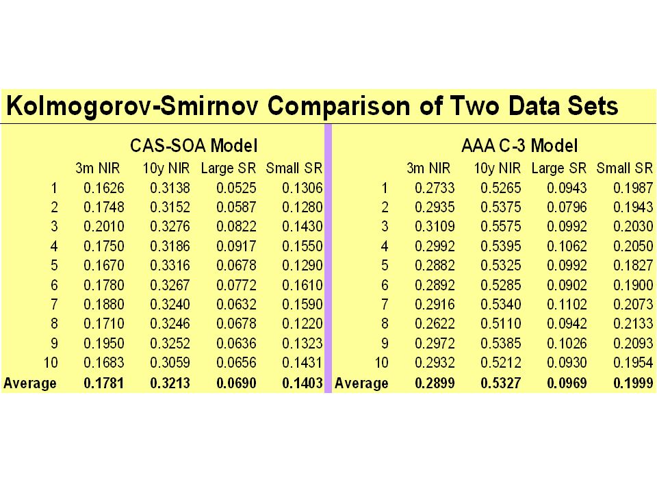
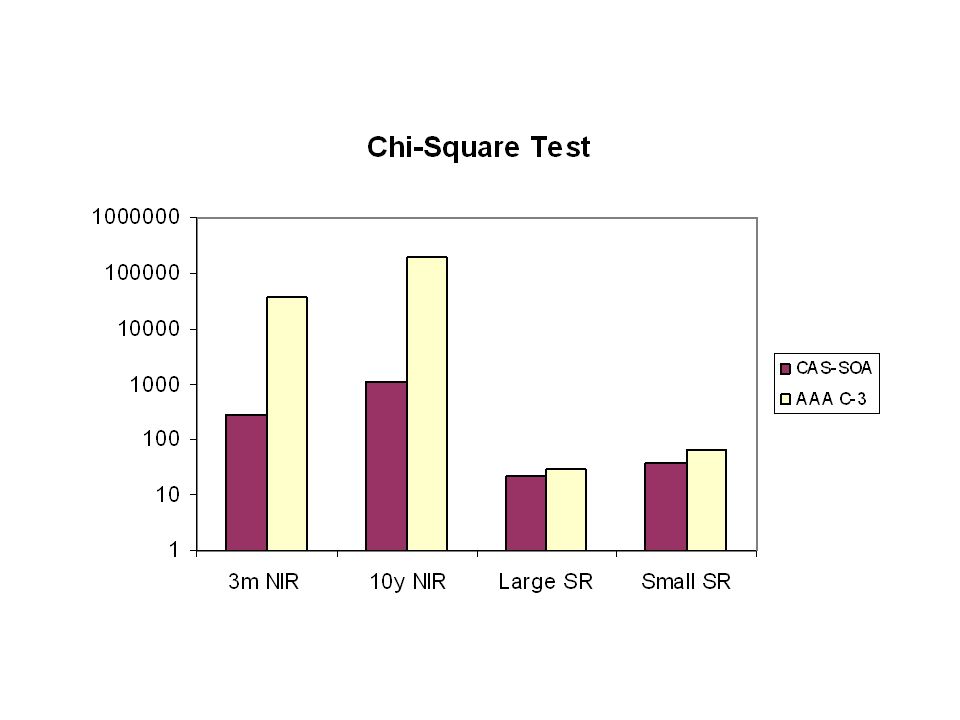
32. Quantification of Model Fit Kolmogorov-Smirnov test Tries to determine if two datasets differ significantly Uses the maximum vertical difference between percentile plots of the data as statistic D Chi-square test Take the squared difference between observed frequency (O) and the expected frequency (E), and then divided by the expected frequency

36. Summary of Differences Kolmogorov-Smirnov test Statistic D of CAS-SOA model is smaller than that of AAA C-3 model Chi-square test For nominal interest rate, the Chi-square value of CAS-SOA model is smaller than that of AAA C-3 model For small stock returns, both models are rejected at significant level of 0.025 while accepted at level of 0.1 For large stock returns, both models are rejected at significant level of 0.05 while accepted at level of 0.1

37. How to Obtain Models CAS-SOA model is posted on the following sites: http://casact.org/research/econ/ http://www.soa.org/ccm/content/areas-of- practice/finance/mod-econ-series-coor-int-rate- scen/http://www.soa.org/ccm/content/areas-of- practice/finance/mod-econ-series-coor-int-rate- scen/ Or contact us at: kahlgrim@ilstu.edukahlgrim@ilstu.edu s-darcy@uiuc.edu gorvett@uiuc.edu AAA model is posted at: http://www.actuary.org/life/phase2.asp