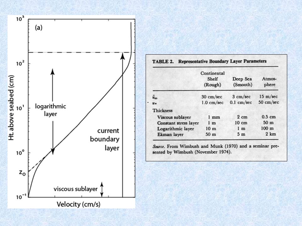
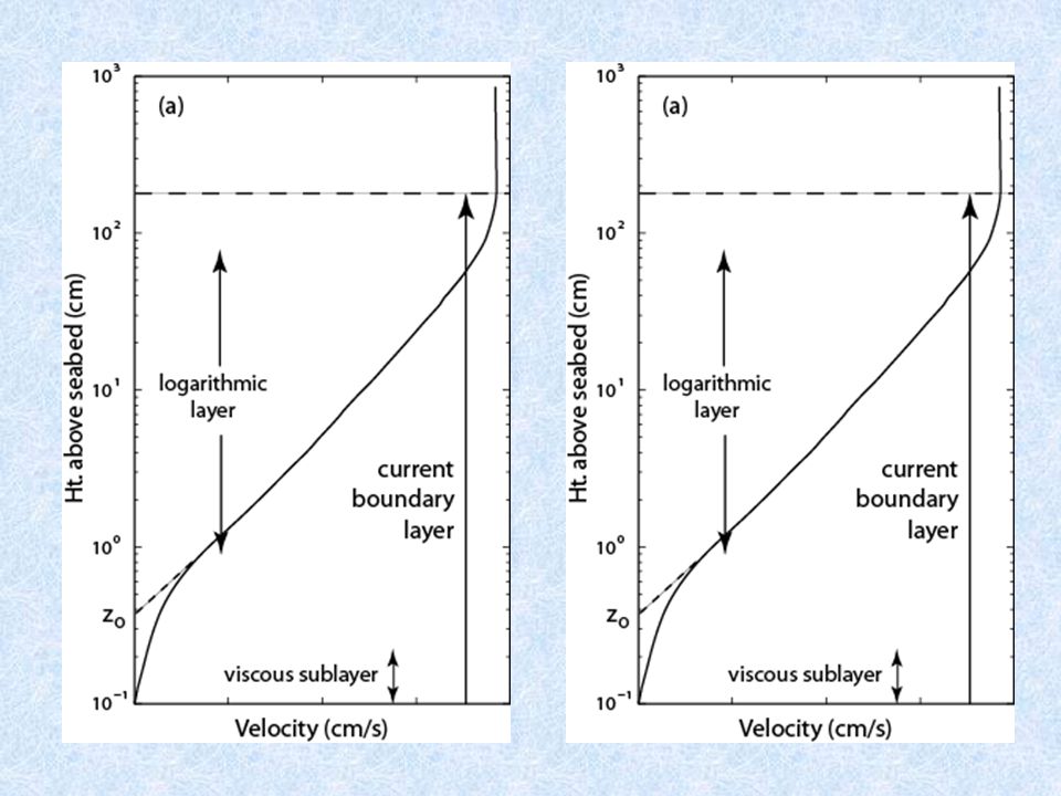
1. Boundary Layer Velocity Profile z ū Viscous sublayer Buffer zone Logarithmic turbulent zone Ekman Layer, or Outer region (velocity defect layer)

2. But first.. a definition:

3. 1. Viscous Sublayer - velocities are low, shear stress controlled by molecular processes As in the plate example, laminar flow dominates, Put in terms of u * integrating, boundary conditions,

4. When do we see a viscous sublayer?  v = f (u *,, k s ) where k s == characteristic height of bed roughness Roughness Re: R * > 70 rough turbulent no viscous sublayer R * < 5 smooth turbulent yes, viscous sublayer

5. 2. Log Layer: Turbulent case, A z is NOT constant in z A z is a property of the flow, not just the fluid To describe the velocity profile we need to develop a profile of A z. Mixing Length formulation Prandtl (1925) which is a qualitative argument discussed in more detail “Boundary Layer Analysis” by Shetz, 1993 Assume that water masses act independently over a distance, l Within l a change in momentum causes a fluctuation to adjacent fluid parcels.

6. At l, Make assumption of isotropic turbulence: |u’| ~ |v’| ~ |w’| Therefore, |u’| ~ |w’| ~ Through the Reynolds Stress formulation, Prandtl Mixing Length Formulation

7. Von Karmen (1930) hypothesized that close to a boundary, the turbulent exchange is related to distance from the boundary. l  z l = Kz where K is a universal turbulent momentum exchange coefficient == von Karmen’s constant. K has been found to be 0.41 Near the bed, in terms of u *

8. Solving for the velocity profile: ln z ū Intercept, b, depends on roughness of the bed - f (R * )

9. Rename b, based on boundary condition: z = z o at ū = 0 Karmen-Prandtl Eq. or Law of the Wall

11. Hydraulic Roughness Length, z o z o is the vertical intercept at which ū z = 0 z o = f ( viscous sublayer, grain roughness, ripples & other bedforms, stratification) This leads to two forms of the Karmen-Prandtl Equation 1) with viscous sublayerHSF 2) without viscous sublayerHRF

13. Can evaluate which case to use with R * where k s == roughness length scale in glued sand, pipe flow experiments k s = D in real seabeds with no bedforms, k s = D 75 in bedforms, characteristic bedform scale k s ~ height of ripples

14. 1. Hydraulically Smooth Flow (HSF) ** boundary layer is turbulent, but there is a viscous sublayer z o is a fraction of the viscous sublayer thickness: Karmen-Prandtl equation becomes: For turbulent flow over a hydraulically smooth boundary

15. 2. Hydraulically Rough Flow (HRF) ** no viscous sublayer z o is a function of the roughness elements Nikaradze pipe flow experiments: Karmen-Prandtl equation becomes: For turbulent flow over a hydraulically rough boundary with no bedforms, no stratification, etc.

16. Notes on z o in HRF Grain Roughness: Nikuradze (1930s) - glued sand grains on pipe flow z o = D/30 Kamphius (1974) - channel flow experiments z o = D/15 Bedforms: Wooding (1973) where H is the ripple height and is the ripple wavelength Suspended Sediment: Smith (1977) z o = f (excess shear stress, and z o from ripples)

17. 3. Hydraulically Transitional Flow (HTF) z o is both fraction of the viscous sublayer thickness and a function of bed roughness. Karmen-Prandtl equation is defined as:

18. Bed Roughness is never well known or characterized, but fortunately not necessary to determine u * If you only have one velocity measurement (at a single elevation), use the formulations above. If you can avoid it.. do so. With multiple velocity measurements, use the “Law of the Wall” to get u * ln z ūzūz

19. To determine  b (or u * ) from a velocity profile: 1. Fit line to data 2. Find slope - 3. Evaluate