1. CHAPTER 7 SYSTEM DESIGN

2. Transmission Types Two types of transmissions: - Link (point to point) - Network -point to multipoint -Mesh -Ring

3. Elements of Link/ Network Design Tx : Operating wavelength ( ), Linewidth (  ), Rise time, Bit-rate, Line format, Power level Fiber : SMF/MMF, Fiber type – SMF28, DSF, etc, Cable loss, Spool length Connection: No. of splice, Splice loss No. of connectors, Connector Loss In Line Devices: Splitter, Filter, Attenuator, Amplifier Insertion loss, Gain Rx : P SEN, P SAT, Rise time

4. The Main Problems Attenuation and Loss Dispersion The Main Question In Digital System - Data Rate -Bit Error Rate In Analog System -Bandwidth -Signal to Noise Ratios

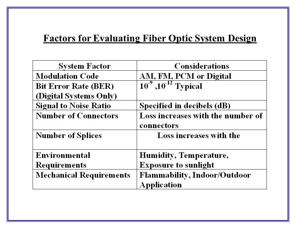
5. Factors for Evaluating Fiber Optic System Design

7. Source LEDs Output Power Modulation Bandwidth Center Wavelength Spectral Width Source Size Laser Diodes Output Power Modulation Bandwidth Center Wavelength, Number of Modes Linewidth

8. Fiber Multimode Fiber Attenuation Multimode Dispersion Chromatic Dispertion Numerical Aperture Core Diameter Single-Mode Fiber Attenuation Chromatic Dispersion Cutoff Wavelength Spot Size

9. Receiver/Photodiode Risetime/Bandwidth Response Wavelength Range Saturation Level Minimum Detection Level

10. Sample Link OA TX RX OA Medium and Devices

11. Link Budget Considerations Three budgets: (1)Power Budget (2)Bandwidth or Rise Time Budget (3)Financial Budgets

12. Power Budget Requirements: P TX - P RX = 2l C +  L + SYSTEM MARGIN l C = connector loss  = fiber attenuation P RX > P MIN P RX = Received Power P MIN = Minimum Power at a certain BER P RX = P TX – Total Losses + Total Gain - P MARGIN P TX = Transmitted Power P MARGIN ≈ 6 dB

13. Requirements Cont’d: Loss,L = L IL + L fiber + L conn. + L non-linear + L D L IL = Insertion Loss L fiber = Fiber Loss L conn. = Connector Loss L non-linear = Non-linear Loss L D = Dispersion-equalization penalty L D = 128 (τ * BR) 4 τ = Total delay or dispersion BR= Transmission bit-rate

14. Requirements Cont’d: Gain,G = Gain amp + G non-linear Gain amp = Amplifier Gain G non-linear = Non-linear Gain

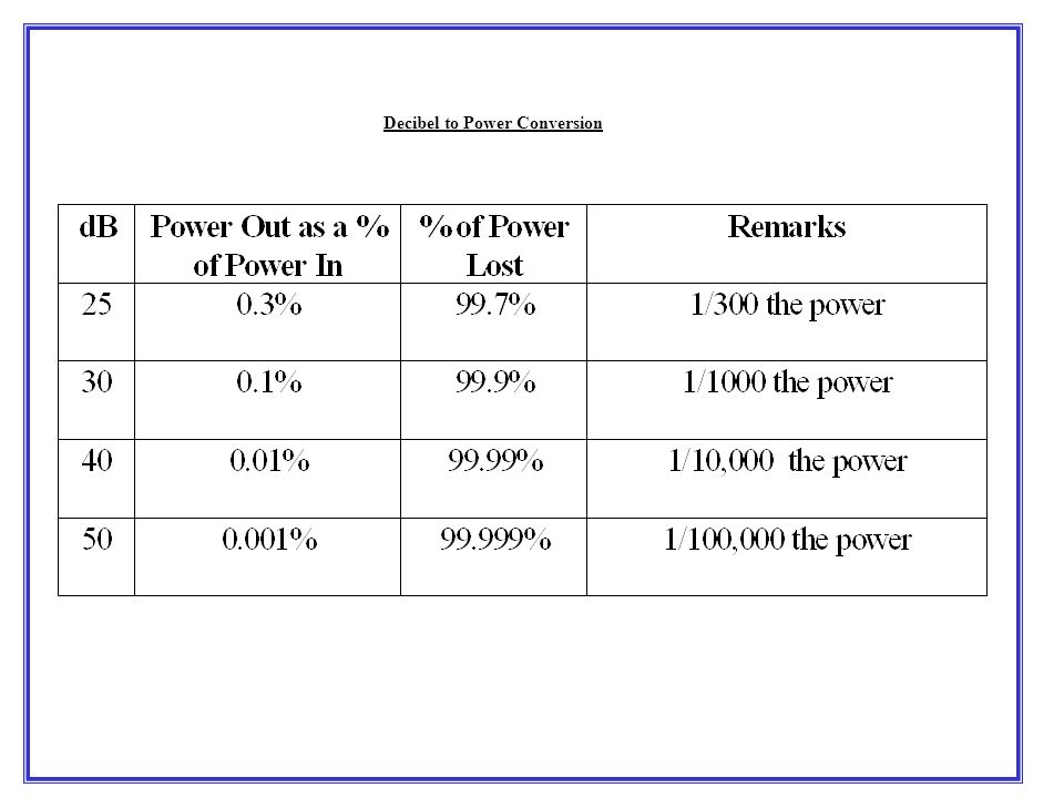
15. dB, dBm, mW dB = 10 log (P 1 /P 2 )

16. Decibel to Power Conversion

19. IS THIS SYSTEM GOOD? Example: Power Budget Measurement P Tx = 0 dBm 185 km P SEN = -28 dBm Splice Attenuation Coefficient,  = 0.25 dB/km Dispersion Coefficient, D = 18 ps/nm-km Number of Splice = 46 Splice Loss = 0.1 dB P Margin = 6 dB L D = ? Connector Loss = 0.2 dB Connector

20. CONCLUSION: BAD SYSTEM!! Simple Calculation…. Fiber Loss = 0.25 dB/km X 185 km = 46.3 dB Splice Loss = 0.1 dB X 46 = 4.6 dB P Margin = 6 dB Total Losses = 46.3 + 4.6 + 0.4 = 51.3 dB Power Budget, P RX < P SEN !! P RX = -57.3 dB P RX = P TX – Total Losses – P Margin = 0 – 51.3 – 6 Connector Loss= 0.2 dB X 2 = 0.4 dB

21. How To Solve? Answer … Place an amplifier But… What is the gain value? ? Where is the location? And…

22. First we calculate the amplifier’s gain.. Gain  P SEN - P RX Gain  -28 – (-57.3) Gain  29.3 dB To make it easy, Gain  30 dB Now…Where to put the amplifier?

23. Three choices available for the location Power Amplifier – At the transmitter Preamplifier – At the receiver In Line – Any point along fiber

24. Let us check one by one… Power Amplifier: P TX + Gain = P OUT 0 + 30 = dBm But is there any power amplifier with 30 dBm P OUT ? NO, IT ISN’T Hence …

25. What about Preamplifier? P OUT received = -57 dBm Remember… Preamplifier with 30 dB available?Yes But, can it take –57 dBm? Typically, NO Hence …

26. Let us check In Line Amplifiers 30 dB gain amplifier available here… But, What value can it take? Typically –30 dBm So… Now, we can find the location…

27. Where is the –30 dBm point? P TX – Loss At That Point = 0 dBm – 30 dB Loss At That Point = -30 dBm 30 =  x Length of That Point Remember  = 0.25, Point Length = 30/0.25 = 120 km But 120 km from Tx, No. of splice = 120/4 = 30 Assume Other Loss = 0, Loss At That Point = Fiber Loss, Splice Loss = 0.1 dB x 30 = 3 dB

28. Also remember connector loss at amplifier and Tx… 2 connectors Connector Loss = 0.2 dB x 3 = 0.6 dB Total Losses = Fiber Loss + Splice Loss + Connector Loss Actually, at 120 km, = 30 + 3 + 0.6 = 33.6 dB 33.6 dB > 30 dB!! NOT GOOD! Now, We have excess of 3.6 dB…Find the distance, Fiber Loss Length = 3.6/0.25 = 14.4 km Good Location = 120 km – 14.4 km = 105.6 km + 1 connector at Tx

29. Let us confirm the answer… At 105.6 km from Tx, Fiber Loss = 0.25 x 105.6 = 26.4 dB No. of Splice at 105.6 km = 105.6/4 =26.4 = 27 Splice Loss = 0.1 x 27 = 2.7 dB Total Losses = 26.4 + 2.7 = 29.1 dB 29.1 dB < 30 dB !! CONFIRM…105.6 KM IS A GOOD LOCATION!! P Tx = 0 dBm 185 km P SEN = -28 dBm Splice Connector 105.6 KM

30. Bandwidth/Rise Time Budget Calculate the total rise times Tx, Fiber, Rx Total Rise time, T sys : T sys =1.1(T TX 2 +T RX 2 +T fiber 2 ) 1/2 Tx Rise Time, T TX = normally given by manufacturer Rx Rise Time, T RX = normally given by manufacturer

31. Bandwidth/Rise Time Budget Calculate fiber rise time, T fiber 2 = T IM 2 + (T CD + T PMD-2 ) 2 + T PMD-1 2 T CD = T mat. + Twg. = D * Δλ * L D G.652 = 18 ps/nm-km D G.652 = Dispersion Coefficient  = Linewidth L = Fiber Length

32. Bandwidth/Rise Time Budget PMD coefficient Coefficient T PMD-1, χ = χ ps/(km) 1/2 Coefficient T PMD-2 = 1.1 * χ ps/nm-km λ in μm λ 2

33. Bandwidth Budget OA TX RX OA Medium and Devices T’ Δτ = T’ - T T

34. What is a good Rise time? For a good reception of signal T sys < 0.7 x Pulse Width (PW) PW = 1/BitRate for NRZ 1/2BitRate for RZ

35. From formula derived before T IM = 0 T CD = 90 ps T PMD-1 = 2.0 ps T PMD-2 = 9 ps Fiber rise time, T fiber 2 = T IM 2 + (T CD + T PMD-2 ) 2 + T PMD-1 2 T fiber 2 = (0) 2 + (90 + 9) 2 + (2) 2 T fiber = 99.02 ps = 0.09902 ns Simple Calculation…. for fiber length = 100km

36. Example: Rise Time Budget Measurement Tx rise time, T TX = 0.1 ns Rx rise time, T RX = 0.1 ns Linewidth(  ) = 0.05 nm Dispersion Coefficient, D = 18 ps/nm-km Assume, Coefficient T PMD-1, χ = 0.2 ps/(km) 1/2 Coefficient T PMD-2 = 0.22 λ = 1.55 μm (1.55) 2 = 0.09 ps/nm-km

37. Total Rise time, T SYS = 1.1  T LS 2 + T PD 2 + T F 2 = 1.1  0.01 + 0.01 + 0.0001 Simple Calculation…. T SYS = 0.16 ns

38. Let say, Bit Rate = STM 4= 622 Mbps Format = NRZ T sys < 0.7 x Pulse Width (PW) Pulse Width (PW) = 1/(622x10 6 ) = 1.6 ns 0.16 ns < 0.7 x 1.6 ns 0.16 ns < 1.1 ns !! Good Rise time Budget!!

39. Let say, Bit Rate = STM 16 = 2.5 Gbps Format = NRZ T sys < 0.7 x Pulse Width (PW) Pulse Width (PW) = 1/(2.5x10 9 ) = 0.4 ns 0.16 ns < 0.7 x 0.4 ns 0.16 ns < 0.28 ns !! Good Rise time Budget!!

40. Let say, Bit Rate = STM 64 = 10 Gbps Format = NRZ T sys < 0.7 x Pulse Width (PW) Pulse Width (PW) = 1/(10x10 9 ) = 1.6 ns 0.16 ns < 0.7 x 0.1 ns 0.16 ns > 0.07 ns !! Bad Rise time Budget!!

41. Budget Summary Option Power Budget Bandwidth Budget Financial A Source (LED vs. LD) Δλ 850nmMediocreBadCheap 1310nmGood Less expensive 1550nmVery good Expensive Modulation Bandwidth LEDNABadCheap LDNAGoodExpensive Output PowerLEDMediocre NA Cheap LDGoodNAExpensive Radiation patternLED (far- field pattern) NA BadCheap LD (Gaussian beam) NAGoodExpensive

42. Budget Summary BFiber Option Power Budget Bandwidth Budget Financial AttenuationMM Mediocre Cheap SMGood Expensive DispersionMM Mediocre Cheap SMGood Expensive Numerical Aperture (NA) MM Mediocre Cheap SMGood Expensive Core DiameterMM Mediocre Cheap SMGood Expensive

43. Budget Summary CReceiver (PIN vs. APD) Option Power Budget Bandwidth Budget Financial Rise time/ Bandwidth PIN Mediocre Cheap APDGood Expensive Response wavelength range PIN Mediocre Cheap APDGood Expensive Saturation LevelPIN Mediocre Cheap APDGood Expensive Minimum detection level PIN Mediocre Cheap APDGood Expensive

44. Sensitivity Analysis - Minimum optical power that must be present at the receiver in order to achieve the performance level required for a given system. Factors will affect this analysis : 1.Source Intensity Noise- Refers to noise generated by the LED or Laser –Phase Noise- the difference in the phases of two optical wavetrains separated by time, cut out of the optical wave –Amplitude Noise - caused by the laser emission process. 2.Fiber Noise –Relates to modal partition noise 3.Receiver Noise –Photodiode, conversion resistor

45. Sensitivity Analysis-contd.. 4.Time Jitter and Intersymbol Interference –Time Jitter - short term variation or instability in the duration of a specified interval –Intersymbol Interference result of other bits interfering with the bit of interest inversely proportional to the bandwidth –Eye diagrams - to see the effects of time jitter and intersymbol interference

46. 5.Bit error rate- main quality criterion for a digital transmission system BER = Q [  I MIN 2 / (4. N 0. B) ] where : N 0 = Noise power spectral density (A 2 /Hz) I MIN = Minimum effective signal amplitude (Amps) B = Bandwidth Q(x) = Cumulative distribution function (Gaussian distribution)

47. Eye Diagrams

48. Signal to Noise Ratio SNR = S/N S - represents the information to be transmitted N - integration of all noise factors over the full system bandwidth SNR (dB) = 10 log 10 (S/N)

49. Modulation Schemes Process of passing information over the communication link : Encoding Transmitting Decoding

50. Types of Modulation Used for Encoding

51. Cost/Performance Considerations Components considerations such as : –Light Emitter Type –Emitter Wavelength –Connector Type –Fiber Type –Detector Type

52. Summary The key factors that determine how far one can transmit over fiber are transmitter optical output power, operating wavelength, fiber attenuation, fiber bandwidth and receiver optical sensitivity. The decibel (dB) is a convenient means of comparing two power levels. The optical link loss budget analyzes a link to ensure that sufficient power is available to meet the demands of a given application. Rise and fall times determine the overall response time and the resulting bandwidth. A sensitivity analysis determines the amount of optical power that must be received for a system to perform properly. Bit errors may be caused by source intensity noise, fiber noise, receiver noise, time jitter and intersymbol interference. The five characteristics of a pulse are rise time, period, fall time, width and amplitude.