1. ISPOL Ocean Turbulence Project Miles McPhee McPhee Research Co. Naches WA USA

2. Objectives Characterize exchanges at or near the ice/ocean interface, representative of the entire ISPOL floe. Pertinent variables include: Turbulent stress Turbulent heat flux Turbulent salt (salinity) flux The ocean velocity profile, including an estimate of geostrophic flow Eddy exchange factors for momentum and scalar variables: eddy viscosity/eddy diffusivity

3. 4 m, T,  C, V 8 m, T, C,  C, V 12 m, T, C, V Sonars RDI 1.2 MHz looking up 600 kHz looking down Sonar, Sontek 500 kHz Phase 1 Deployment– 30 Nov to 25 Dec 2 m thick ice

4. 2 m, T,  C, V 4 m, T, C, V Sonar, Sontek 500 kHz Phase 2 Deployment – Dec 26- Jan 1 1 m thick ice

5. SonTek ADVOcean (5 Mhz) SBE 03 thermometer SBE 07 microstructure conductivity meter SBE 04 conductivity meter SonTek Instrument Cluster

6. Two methods used for fitting ship GPS positions to a differentiable function to obtain velocity: (1)Polynomial fit: all 5-min position vectors in a 1-h time window centered at even half-hour intervals were converted to complex numbers and least-squares fitted to complex second-order polynomial. The derivative provides a continuous velocity record. (2)Complex demodulation: fits all of the data over a 1-day time window to a position function including mean velocity and clockwise and anticlockwise oscillating components at the inertial and diurnal frequencies. Done every 90 minutes

9. These are tidal components in the ice motion– they correspond to the ocean tidal current only if the ice drifts passively with the tide.

14. Site A Deployment 1: 1 mast with 2 turbulence clusters nominally 6 and 10 m depth (4 and 8 m below the ice/ocean interface) with upward/downward looking RDI ADPs From 336.75 to 343.75 Site A Deployment 2: Same mast as Deployment 1, plus 2 nd mast with 1 turbulence cluster at 4 m depth (2 m from interface) and 500 kHz Sontek ADP From 345.00 to 353.375 Site A Deployment 3: 1 mast with 3 turbulence clusters nominally 4, 8, and 12 m depth (2, 4, 10 m below the ice/ocean interface) with upward/downward looking RDI ADPs, plus the Sontek ADP deployed separately in the same hydrohole. From 354.75 to 360.25 Site B Deployment: 1 mast with 2 turbulence clusters nominally 2 and 4 m depth (1 and 2 m below the ice/ocean interface) with the Sontek ADP on the bottom of the mast. From 362.625 to 367.50

15. Site A-1 Site A-2 15-minute realizations (covariance calculations) averaged for 3 hours.

16. Site A-3 Site B

17. Site A-1

18. Site A-2

19. Site A-3

20. Site B

21. Site A-1

22. Site A-2

23. Site A-3

24. Site B

27. Relative current, TIC 1

30. Relative current, TIC 2

34. Day 363.50 Cluster u * U/u * 1 0.0085 4.5 2 0.0135 4.1

35. Relative current, TIC 2

36. Day 365.25 Cluster u * U/u * 1 0.0048 17.9 2 0.0059 16.6

38. For near neutral stability, the mixing length near the ice/water interface is limited by both the distance from the interface (geometric scale) and by rotation (planetary scale). The former is  |z|, while in my similarity approach the latter limit is  * u *. /|f|, where f is the Coriolis parameter. So, in this idealized view, for an instrument cluster at |z|= 2 m where z is measured from the interface,  should look like:

39. From turbulence mast data obtained during ISPOL in Dec 2004, the mixing length was calculated from the spectral peaks for each 3-hr average, and plotted as a scatter diagram versus the local friction velocity. If the geometric surface layer scale,  |z|, controlled the scale, then for example, at 2 m and 4 m from the interface, the mixing length would follow the yellow and blue horizontal lines respectively. If instead, dynamic boundary layer scaling dominated, the relationship would be indicated by the dashed red line. The heavy dot-dash line is a least-squares regression (through the origin) of versus u * with light dashed lines indicating confidence limits. The slope is thus indistinguishable from  * /f.

40. Green circles: law of the wall, median value of log (z 0 ) shown with error bars indicating 95% confidence interval for the median based on quartile limits. Red squares: mixing length method, which includes as a measured parameter the length scale inversely proportional to the wavenumber at the peak of the area-preserving w spectrum.

41. Treat velocity vectors as complex numbers: V=u+iv

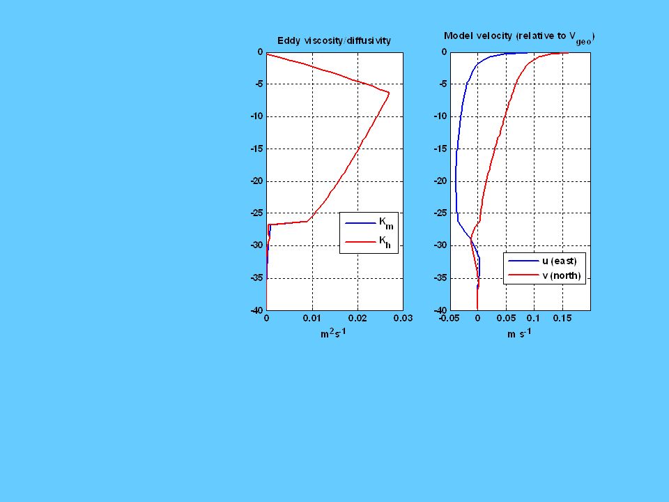
49. For each 3-h segment of data, run the steady model forced to agree with the current at 20 m, using the interpolated T/S structure in the upper ocean, adjusted to agree with upper cluster values. For each sample, calculate the nondimensional profile (with respect to the 30 m level) and compare the model average with measured.

50. Green circles: law of the wall, median value of log (z 0 ) shown with error bars indicating 95% confidence interval for the median based on quartile limits. Red squares: mixing length method, which includes as a measured parameter the length scale inversely proportional to the wavenumber at the peak of the area-preserving w spectrum.

55. Summary The ocean turbulence data were characterized by much temporal variability and undersurface heterogeneity. For the purpose of estimating exchange properties for the entire floe, a relatively simple, steady state upper ocean model was applied to each 3-h average, for a range of roughness values. The modeled angular shear between 10 and 30 m was compared with observations, and from this, z 0 = 0.05 m emerged as a representative value. The model then provides interface values for the friction velocity, heat flux, salt flux. It additionally estimates eddy viscosity/diffusivity, and velocity through the boundary layer, along with estimates of the undisturbed geostrophic velocity.