Download presentation
Presentation is loading. Please wait.

1
Splines Vida Movahedi January 2007

2
Outline Piecewise polynomials Splines Two approaches B-splines
Multivariate functions Examples

3
What problem splines solve?
In the simplest situation, one is given points (ti, yi) and is looking for a piecewise polynomial function f that satisfies f(ti)=yi , all i, more or less. Exact fit Interpolation Approximate fit least squares approximation or smoothing splines Or we have a complex function g that we want to approximate with a piecewise polynomial function f that satisfies f(ti)=g(ti) , all i, more or less.
 and is looking for a piecewise polynomial function f that satisfies f(ti)=yi , all i, more or less. Exact fit Interpolation. Approximate fit least squares approximation or smoothing splines. Or we have a complex function g that we want to approximate with a piecewise polynomial function f that satisfies f(ti)=g(ti) , all i, more or less.")
5
Why polynomials? Easy evaluation, differentiation, and integration
If done properly, the work needed for data fitting grows only linearly with the number of data points.

6
Definition of Polynomial of order n
Note that a polynomial of order n has degree<n The set of all polynomials of order n forms a linear space <n: linear space of polynomials of order n

7
Why piecewise polynomials?
Jackson’s Theorem: If g has r continuous derivatives on [a..b] and n> r+1, then The only way to make the error small is to make (b-a)/ (n-1) small partitioning [a..b] using piecewise polynomial approximation. It is usually much more efficient to make (b-a) small than to increase n. This is the justification for piecewise polynomial approximation.
/ (n-1) small partitioning [a..b] using piecewise polynomial approximation. It is usually much more efficient to make (b-a) small than to increase n. This is the justification for piecewise polynomial approximation.")
8
Why not higher order polynomials?
We expect the error between the function g and the polynomial approximation pn on n sites to decrease when n increases. If the sites are uniformly spaced, it can be shown that this is not true and the interpolation error increases with n for some examples. It is shown that choosing the sites as the zeros of the Chebyshev polynomial of degree n can lead to much decreasing interpolation error with increasing n. For some examples, the error, while decreasing, decreases far too slowly.

9
What is a spline? An interval [a..b] is subdivided into sufficiently small intervals [j.. j+1], with a=1<…<l+1=b, On each such interval, a polynomial pj of relatively low degree can provide a good approximation to g. This can even be done in such a way that the polynomial pieces blend smoothly, i.e. so that the resulting composite function s(x) that equals pj(x) for x[j j+1] , all j , has several continuous derivatives. Any such smooth piecewise polynomial function is called a spline.
![What is a spline An interval [a..b] is subdivided into sufficiently small intervals [j.. j+1], with a=1<…<l+1=b,](http://slideplayer.com/slide/7917554/25/images/9/What+is+a+spline+An+interval+%5Ba..b%5D+is+subdivided+into+sufficiently+small+intervals+%5B%EF%81%B8j..+%EF%81%B8j%2B1%5D%2C+with+a%3D%EF%81%B81%3C%E2%80%A6%3C%EF%81%B8l%2B1%3Db%2C.jpg "On each such interval, a polynomial pj of relatively low degree can provide a good approximation to g. This can even be done in such a way that the polynomial pieces blend smoothly, i.e. so that the resulting composite function s(x) that equals pj(x) for x[j j+1] , all j , has several continuous derivatives. Any such smooth piecewise polynomial function is called a spline.")
10
Continuous 1st derivative Continuous 2nd derivative

11
Two major approaches The ppform: Use of piecewise polynomials
The B-form: Use of Basis functions

12
ppform More efficient when evaluating the spline extensively
The ppform of a polynomial spline of order k provides a description in terms of its breaks 1,…,l+1 and the local polynomial coefficients cji of its l pieces. For linear approximation

13
Example g(x)=sin(x) >> x=0:0.6:pi; y=sin(x); >> figure; plot (x,y, 'o') >> sp=spapi(2,x,y); >> hold on; fnplt(sp); >> pp=sp2pp(sp); >>fnbrk(pp) The input describes a ppform breaks(1:l+1) Columns 1 through 5 Column 6 3.0000 coefficients(d*l,k) pieces number l 5 order k 2 dimension d of target 1 Breaks (interpolation) Interpolating spline of order 2 The ppform provides the coefficients for each of the polynomial pieces between the breaks. In the above example the coefficients for each of the lines is provided.
; >>fnbrk(pp) The input describes a ppform. breaks(1:l+1) Columns 1 through Column coefficients(d*l,k) pieces number l. 5. order k. 2. dimension d of target. 1. Breaks (interpolation) Interpolating spline of order 2. The ppform provides the coefficients for each of the polynomial pieces between the breaks. In the above example the coefficients for each of the lines is provided.")
14
The B-form Useful during construction of a spline
The B-form describes a spline as a weighted sum of B-splines of the required order k, with their number n>k-1+l Each Bj,k is defined on an interval [tj..tj+k] and is zero elsewhere. tj are called knots and are provided based on the smoothness required (breaks, but sometimes repeated!) B-splines are functions that:
 B-splines are functions that:")
15
(uniform spacing between knots)
Example B-splines of order 2 (uniform spacing between knots)
")
16
Note that in ppform, we had 6 breaks, and 10 coefficients.
Example (cont.) >> fnbrk(sp) The input describes a B-form knots(1:n+k) Columns 1 through 7 Column 8 3.0000 coefficients(d,n) number n of coefficients 6 order k 2 dimension d of target 1 Note that in ppform, we had 6 breaks, and 10 coefficients.
 >> fnbrk(sp) The input describes a B-form. knots(1:n+k) Columns 1 through Column coefficients(d,n) number n of coefficients. 6. order k. 2. dimension d of target. 1. Note that in ppform, we had 6 breaks, and 10 coefficients.")
17
Control Points aj are called the control points
If B are B-splines aj are de Boor control points If B are Bezier splines aj are Bezier control points Bezier Control Points de Boor Control Points for B-splines

18
Why B-splines? Composed of (n-k+2) curves of k-order joined Ck-2 continuously at knot values (t0,…,tn+k) smoothness and continuity Each point is affected by k control points Each control point affects k segments local controllability Inside convex hull Built-in boundedness does not shoot to infinity (unlike Bezier) Affine invariance Any degree of detail desired Generative nature
 Affine invariance. Any degree of detail desired Generative nature.")
19
Uniform B-splines If the knots are equi-spaced, for a given order k, the splines are simply shifted copies of one another. Linear B-splines (k=2) Cubic B-splines (k=4)
 Cubic B-splines (k=4)")
20
knot multiplicity Knots are a sequence of breaks, sometimes repeated!
The rule is Knot multiplicity + condition multiplicity = order For example, for a B-spline of order k=3 Simple knot smoothness_cond=2 continuity of function and first derivative Double knot smoothness_cond= 1 just continuity Triple knot No condition function can even be discontinuous

21
Multivariate Functions
If f is a function of x, and g is a function of y, then their tensor-product p(x,y):=f(x)g(y) is a function of x and y. For example for a bivariate spline of order h in x and k in y, we have: Knot sequences s= (s1,…, sm+h) t= (t1,…,tn+k) Coefficients (aij:i=1..m, j=1..n)
:=f(x)g(y) is a function of x and y. For example for a bivariate spline of order h in x and k in y, we have: Knot sequences. s= (s1,…, sm+h) t= (t1,…,tn+k) Coefficients (aij:i=1..m, j=1..n)")
22
Chord-Length Method The knots must be non-decreasing!
So, what should we do for closed curves?! [1,4,7,10,6,3] not acceptable t: new variable , increasing as we follow the contour x and y will be functions of t

23
Representing Image Contours
Contour from Paco’s grouping algorithm

24
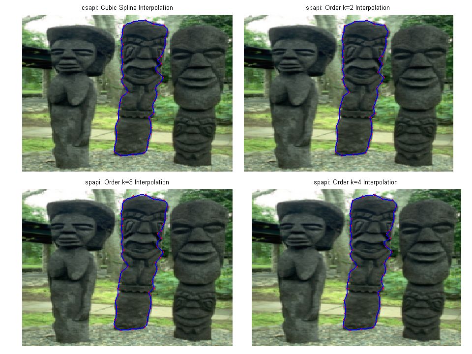
Interpolation unit step: 50

26
Interpolation unit step: 10

28
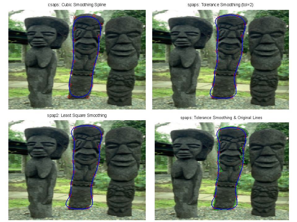
Smoothing unit step: 50

30
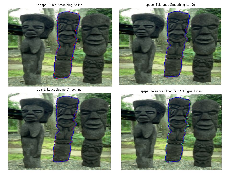
Smoothing unit step: 10

32
Note the corners At least one sample from each line? Unit step: 20

34
Questions? Which method is better? Interpolation or smoothing?
What order? Linear, cubic, …? How can we calculate the error? Should we compare with the original lines? Or with image?

35
References Matlab Spline Toolbox
Carl de Boor, A Practical Guide to Splines, Springer, 2001. ‘An Interactive Introduction to Splines’, Cohen, F.S.; Wang, J.Y. , “Part I: Modeling Image Curves Using Invariant 3-D Object Curve Models- A Path to 3-D Recognition and Shape Estimation from Image Contours”, IEEE Transactions on Pattern Analysis and Machine Intelligence, vol. 16, no. 1, Jan Miroslaw Kuc, COSC Project report: “Representing Image Contours with Splines”, Jan. 2005 Branka Otasevic, COSC Project report, Winter 1999.

Similar presentations