1. Combining Statistical Language Models via the Latent Maximum Entropy Principle Shaojum Wang, Dale Schuurmans, Fuchum Peng, Yunxin Zhao

2. Abstract Simultaneously incorporate various aspects of natural language –Local word interaction, syntactic structure, semantic document information Latent maximum entropy (LME) principle –Which allows relationships over hidden features to be effectively captured in a unified model –Local lexical models (N-gram models) –Global document-level semantic models (PLSA)

3. Introduction There are various kinds of language models that can be used to capture different aspects of natural language regularity –Markov chain (N-gram) models effectively capture local lexical regularities in text –Smoothed N-gram: estimating rare events –Increase the order of an N-gram to capture longer range dependencies in natural language  curse of dimensionality (Rosenfeld)

4. Introduction –Structural language model effectively exploits relevant syntactic regularities to improve the perplexity score of N-gram models –Semantic language model exploits document-level semantic regularities to achieve similar improvements Although each of these language models outperforms simple N-grams, they each only capture specific linguistic phenomena

5. Introduction Several techniques for combining language models: –Linear interpolation: each individual model is trained separately and then combined by a weighted linear combination –Maximum entropy: it model distributions over explicitly observed features There are many hidden semantic and syntactic information in natural language

6. Introduction Latent maximum entropy (LME) principle extends ME to incorporate latent variables Let X  X denote the complete data, Y  Y be the observed incomplete data and Z  Z be the missing data.  X = (Y, Z) The goal of ME is to find a probability model that matches certain constraints in the observed data while otherwise maximizing entropy

7. Maximum Entropy construct separate models –Build a single, combined model, which attempts to capture all the information provided by tie various knowledge sources The intersection of all the constraints, if not empty, contains a (typically infinite) set of probability function, which are all consistent with the knowledge sources The second step in the ME approach is to choose, from among the functions in that set, that function which has the highest entropy (i.e. the “flattest” function)

8. An example Assume we wish to estimate P(“BANK”|h), one estimate may be provided by a conventional bigram Features

9. An example Consider one such equivalence class, say, the one where the history ends in “THE”. The bigram assigns the same probability estimate to all events in that class where is the does the …… the [1]

10. An example Another estimate may be provided by a particular trigger pair, say (LOAN,BANK) –Assume we want to capture the dependency of “BANK” on whether or not “LOAN” occurred before it in the same document. Thus a different partition of the event space will be added, as in Table IV –Similarly to the bigram case, consider now one such equivalence class, say, the one where “LOAN” did occur in the history. The trigger component assigns the same probability estimate to all events in that class

11. …loan…the…loan…of Features

12. An example Consider the bigram, under ME, we no longer insist that P(BANK|h) always have the same value (K {THE,BANK} ) whenever the history ends in “THE” Rather, we only require that P COMBINED (BANK|h) be equal to (K {THE,BANK} ) on average in the training data Equation [1] is replaced by where E stands for an expectation [2]

13. An example Similarly, we require that P COMBINED (BANK|h) be equal to K {BANK,LOANvh} on average over those histories that contain occurrences of “LOAN” [3]

14. Information sources as constraint functions We can view each information source as defining a subset (or many subsets) of the event space (h,w) We can define any subset S of the event space, and any desired expectation K, and impose the constraint: The subset S can be specified by an index function, also called selector function, f s : [4]

15. Information sources as constraint functions so Equation [4] becomes: [5]

16. Maximum Entropy The ME Principle (Jaynes, 1975; Kullback, 1959) can be stated as follows –1. Reformulate the different information sources as constraints to be satisfied by the target (combined) estimate –2. Among all probability distributions that satisfy these constraints, choose the one that has the highest entropy

17. Maximum Entropy Given a general event space {x}, to derive a combined probability function P(x), each constraint i is associated with a constraint function f i (x) and a desired expectation K i The constraint is then written as : [6]

18. LME Given features f 1,…,f N specifying the properties we would like to match in the data, select a joint model p* from the set of possible probability distributions that maximizes the entropy

19. LME Intuitively, the constraints specify that we require the expectations of f i (X) in the joint model to match their empirical expectations on the incomplete data Y – f i (X) = f i (Y, Z) When the features only depend on the observable data Y, the LME is equivalent to ME

20. Regularized LME (RLME) ME principle are subject to errors due to the empirical data, especially in a very sparse domain –Add a penalty to the entropy of the joint model

21. A Training Algorithm Assume we have already selected the features f 1,…f N from the training data Restrict p(x) to be an exponential model

22. A Training Algorithm Intimately related to finding locally maximum a posteriori (MAP) solutions: –Given a penalty function U over errors a, an associated prior U* on can be obtained by setting U* to the convex conjugate of U –e.g., given a quadratic penalty, the convex conjugate can be determined by setting ; which specifies a Gaussian prior on

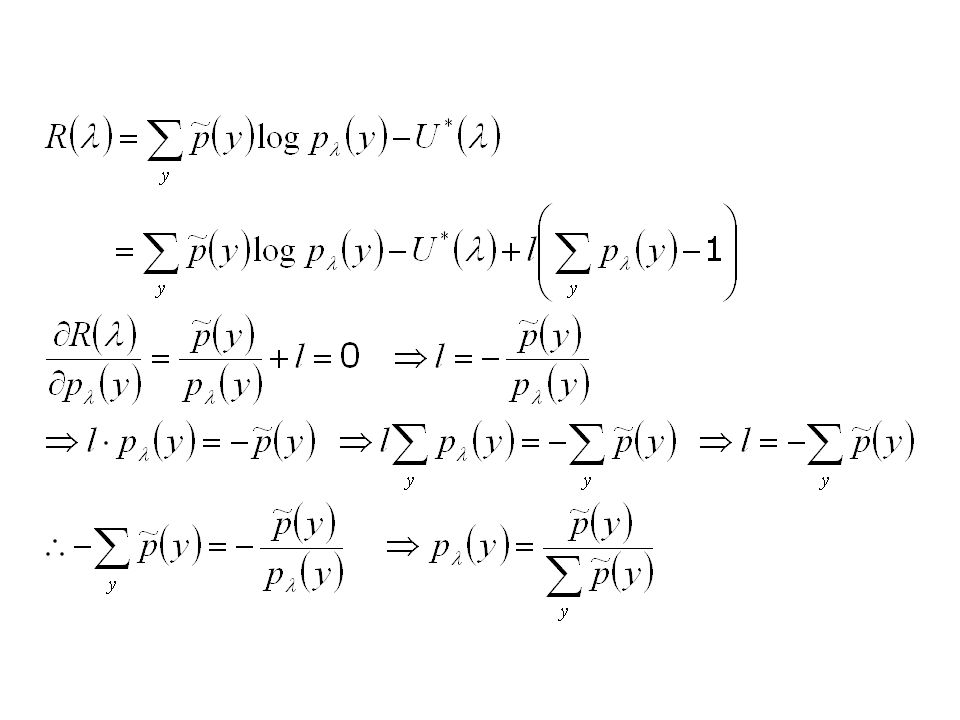
23. A Training Algorithm –Then, given a prior U*, the standard MAP estimate maximizes the penalized log-likelihood Our key result is that locally maximizing R( ) is equivalent to satisfying the feasibility constraints (2) of the RLME principle

24. A Training Algorithm THEOREM 1. –Under the log-linear assumption, locally maximizing a posterior probability of log-linear models on incomplete data is equivalent to satisfying the feasibility constraints of the RLME principle. That is, the only distinction between MAP and RLME in log- linear models is that, among local maxima (feasible solutions), RLME selects the model with the maximum entropy, whereas MAP selects the model with the maximum posterior probability

25. A Training Algorithm R-EM-IS, which employs an EM algorithm as an outer loop, but uses a nested GIS/IIS algorithm to perform the internal M step Decompose the penalized log-likelihood function R( ): This is a standard decomposition used for deriving EM

26. A Training Algorithm For log-linear models:

27. A Training Algorithm LEMMA 1.

28. R-EM-IS algorithm

29. THEOREM 2.

31. R-ME-EM-IS algorithm

32. Combining N-gram and PLSA Models

33. Tri-gram portion

34. PLSA portion

35. Efficient Feature Expectation and Inference Sum-product algorithm: Normalization constant: Feature expectations:

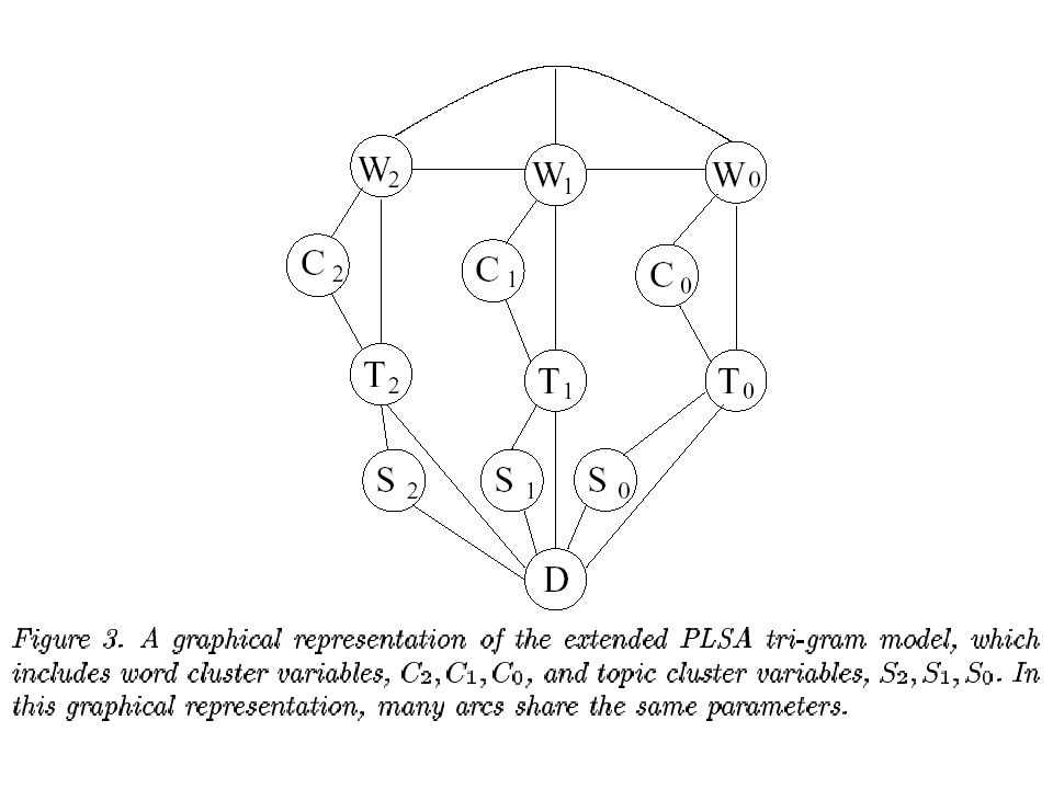
36. Semantic Smoothing Add node C as word cluster between each topic node and word node. –|C| = 1, maximum smoothing –|C| = |V|, no smoothing (|V| is the vocabulary size) Add node S as document cluster between topic node and document node –|S| = 1, over-smoothed –|S| = |D|, no smoothing (|D| is the number of documents) W|C|TW|C|T T|S|DT|S|D

37. Computation in Testing

38. Experimental Evaluation Training Data: –NAB : 87000 documents, 1987~1989, 38M words Vocabulary size, |V|, is 20000, the most frequent words of the training data Testing Data: –325000 words, 1989 Evaluation:

39. Experimental design Baseline: Tri-gram with GT smoothing, perplexity is 105 R-EM-IS procedure: EM iteration is 5, IIS loop iteration is 20 Feasible solution: initialized the parameters to zero and executed a single run of R-EM-IS RLME and MAP: use 20 random starting points for

40. Simple tri-gram There are no hidden variables, MAP, RLME and single run of R-EM-IS all reduce to the same standard ME principle Perplexity score is 107

41. Tri-gram + PLSA |T| = 125 95 91 89

43. Add word cluster 89 93 84

44. Add topic cluster 90 87

45. Add word and topic clusters (1/2) 82

46. Add word and topic clusters (2/2)

47. Experiment summarizes

48. Extensions LSA: Perplexity = 97

49. Extensions Raising LSA portion’s contribution to some power and renormalizing Perplexity = 82, equal to the best results using RLME