1. Jake Blanchard University of Wisconsin Spring 2006

2.  Monte Carlo approaches use random sampling to simulate physical phenomena  They have been used to simulate particle transport, risk analysis, reliability of components, molecular modeling, and many other areas

3.  Consider a cantilever beam with a load (F) applied at the end  Assume that the diameter (d) of the beam cross section, the load (F), and the elastic modulus (E) of the beam material vary from beam to beam (L is constant – 10 centimeters)  We need to know the character of the variations in the displacement (  ) of the end of the beam

4. F d

5.  If F is the only random variable and F has, for example, a lognormal distribution, then the deflection will also have a lognormal distribution  But if several variables are random, then the analysis is much more complication

6.  Assume/determine a distribution function to represent all input variables  Sample each (independently)  Calculate the deflection from the formula  Repeat many times to obtain output distribution

7.  Assume E, d, and F are random variables with uniform distributions Variablea (min value)b (max value) F (N)1,0001,050 d (m)0.010.011 E (GPa)200210

8. length=0.1 force=1000+50*rand(1) diameter=0.01+rand(1)*0.001 modulus=200e9+rand(1)*10e9 inertia=pi*diameter^4/64 displacement=force*length^3/3/modulus/inertia

9. length=0.1 nsamples=100000 for i=1:nsamples force=1000+50*rand(1); diameter=0.01+rand(1)*0.001; modulus=200e9+rand(1)*10e9; inertia=pi*diameter^4/64; displacement(i)=force*length^3/3/modulus/inertia; end

10. length=0.1 nsamples=100000 force=1000+50*rand(nsamples,1); diameter=0.01+rand(nsamples,1)*0.001; modulus=200e9+rand(nsamples,1)*10e9; inertia=pi*diameter.^4/64; displacement=force.*length^3/3./modulus./inertia;

11.  The direct approach is much faster  For 100,000 samples the loop takes about 3.9 seconds and the direct approach takes about 0.15 seconds (a factor of almost 30  I used the “tic” and “toc” commands to time these routines

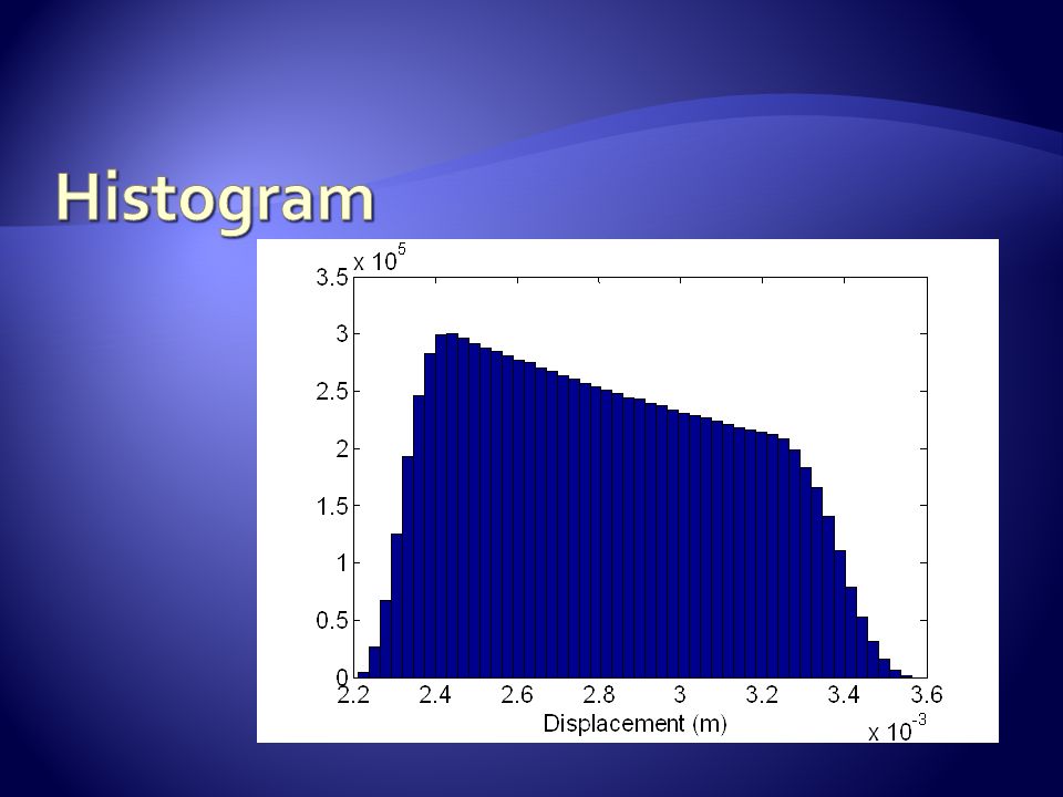
12.  Mean  Standard deviation  histogram min(displacement) max(displacement) mean(displacement) std(displacement) hist(displacement, 50)