Download presentation
Presentation is loading. Please wait.

1
Inferring gene regulatory networks from transcriptomic profiles Dirk Husmeier Biomathematics & Statistics Scotland

2
Overview Introduction Application to synthetic biology Lessons from DREAM

3
Network reconstruction from postgenomic data

4
Accuracy Computational complexity Methods based on correlation and mutual information Conditional independence graphs Mechanistic models Bayesian networks

5
Accuracy Computational complexity Methods based on correlation and mutual information Conditional independence graphs Mechanistic models Bayesian networks

6
direct interaction common regulator indirect interaction co-regulation Pairwise associations do not take the context of the systeminto consideration Shortcomings

7
Accuracy Computational complexity Methods based on correlation and mutual information Conditional independence graphs Mechanistic models Bayesian networks

8
Conditional Independence Graphs (CIGs) 2 2 1 1 Direct interaction Partial correlation, i.e. correlation conditional on all other domain variables Corr(X 1,X 2 |X 3,…,X n ) Problem: #observations < #variables Covariance matrix is singular strong partial correlation π 12 Inverse of the covariance matrix
 Problem: #observations < #variables Covariance matrix is singular strong partial correlation π 12 Inverse of the covariance matrix.")
9
Accuracy Computational complexity Methods based on correlation and mutual information Conditional independence graphs Mechanistic models Bayesian networks

10
Model Parameters q Probability theory Likelihood

11
1) Practical problem: numerical optimization q 2) Conceptual problem: overfitting ML estimate increases on increasing the network complexity
 Practical problem: numerical optimization q 2) Conceptual problem: overfitting ML estimate increases on increasing the network complexity")
12
Overfitting problem True pathway Poorer fit to the data Equal or better fit to the data

13
Regularization E.g.: Bayesian information criterion Maximum likelihood parameters Number of parameters Number of data points Data misfit term Regularization term

14
Complexity LikelihoodBIC

15
Model selection: find the best pathway Select the model with the highest posterior probability: This requires an integration over the whole parameter space:

16
Problem: huge computational costs q

17
Accuracy Computational complexity Methods based on correlation and mutual information Conditional independence graphs Mechanistic models Bayesian networks

18
Friedman et al. (2000), J. Comp. Biol. 7, 601-620 Marriage between graph theory and probability theory

19
Bayes net ODE model

20
Model Parameters q Bayesian networks: integral analytically tractable!

21
UAI 1994

22
[A]= w1[P1] + w2[P2] + w3[P3] + w4[P4] + noise Linearity assumption A P1 P2 P4 P3 w1 w4 w2 w3
![[A]= w1[P1] + w2[P2] + w3[P3] + w4[P4] + noise Linearity assumption A P1 P2 P4 P3 w1 w4 w2 w3](http://images.slideplayer.com/25/7895462/slides/slide_22.jpg "[A]= w1[P1] + w2[P2] + w3[P3] + w4[P4] + noise Linearity assumption A P1 P2 P4 P3 w1 w4 w2 w3")
23
t1t1 t2t2 t3t3 t4t4 t5t5 t6t6 t7t7 t8t8 t9t9 t 10 X (1) X 1,1 X 1,2 X 1,3 X 1,4 X 1,5 X 1,6 X 1,7 X 1,8 X 1,9 X 1,10 X (2) X 2,1 X 2,2 X 2,3 X 2,4 X 2,5 X 2,6 X 2,7 X 2,8 X 2,9 X 2,10 X (3) X 3,1 X 3,2 X 3,3 X 3,4 X 3,5 X 3,6 X 3,7 X 3,8 X 3,9 X 3,10 X (4) X 4,1 X 4,2 X 4,3 X 4,4 X 4,5 X 4,6 X 4,7 X 4,8 X 4,9 X 4,10 Homogeneity assumption
 X 1,1 X 1,2 X 1,3 X 1,4 X 1,5 X 1,6 X 1,7 X 1,8 X 1,9 X 1,10 X (2) X 2,1 X 2,2 X 2,3 X 2,4 X 2,5 X 2,6 X 2,7 X 2,8 X 2,9 X 2,10 X (3) X 3,1 X 3,2 X 3,3 X 3,4 X 3,5 X 3,6 X 3,7 X 3,8 X 3,9 X 3,10 X (4) X 4,1 X 4,2 X 4,3 X 4,4 X 4,5 X 4,6 X 4,7 X 4,8 X 4,9 X 4,10 Homogeneity assumption")
24
Accuracy Computational complexity Methods based on correlation and mutual information Conditional independence graphs Mechanistic models Bayesian networks

25
Example: 4 genes, 10 time points t1t1 t2t2 t3t3 t4t4 t5t5 t6t6 t7t7 t8t8 t9t9 t 10 X (1) X 1,1 X 1,2 X 1,3 X 1,4 X 1,5 X 1,6 X 1,7 X 1,8 X 1,9 X 1,10 X (2) X 2,1 X 2,2 X 2,3 X 2,4 X 2,5 X 2,6 X 2,7 X 2,8 X 2,9 X 2,10 X (3) X 3,1 X 3,2 X 3,3 X 3,4 X 3,5 X 3,6 X 3,7 X 3,8 X 3,9 X 3,10 X (4) X 4,1 X 4,2 X 4,3 X 4,4 X 4,5 X 4,6 X 4,7 X 4,8 X 4,9 X 4,10
 X 1,1 X 1,2 X 1,3 X 1,4 X 1,5 X 1,6 X 1,7 X 1,8 X 1,9 X 1,10 X (2) X 2,1 X 2,2 X 2,3 X 2,4 X 2,5 X 2,6 X 2,7 X 2,8 X 2,9 X 2,10 X (3) X 3,1 X 3,2 X 3,3 X 3,4 X 3,5 X 3,6 X 3,7 X 3,8 X 3,9 X 3,10 X (4) X 4,1 X 4,2 X 4,3 X 4,4 X 4,5 X 4,6 X 4,7 X 4,8 X 4,9 X 4,10")
26
t1t1 t2t2 t3t3 t4t4 t5t5 t6t6 t7t7 t8t8 t9t9 t 10 X (1) X 1,1 X 1,2 X 1,3 X 1,4 X 1,5 X 1,6 X 1,7 X 1,8 X 1,9 X 1,10 X (2) X 2,1 X 2,2 X 2,3 X 2,4 X 2,5 X 2,6 X 2,7 X 2,8 X 2,9 X 2,10 X (3) X 3,1 X 3,2 X 3,3 X 3,4 X 3,5 X 3,6 X 3,7 X 3,8 X 3,9 X 3,10 X (4) X 4,1 X 4,2 X 4,3 X 4,4 X 4,5 X 4,6 X 4,7 X 4,8 X 4,9 X 4,10 Standard dynamic Bayesian network: homogeneous model
 X 1,1 X 1,2 X 1,3 X 1,4 X 1,5 X 1,6 X 1,7 X 1,8 X 1,9 X 1,10 X (2) X 2,1 X 2,2 X 2,3 X 2,4 X 2,5 X 2,6 X 2,7 X 2,8 X 2,9 X 2,10 X (3) X 3,1 X 3,2 X 3,3 X 3,4 X 3,5 X 3,6 X 3,7 X 3,8 X 3,9 X 3,10 X (4) X 4,1 X 4,2 X 4,3 X 4,4 X 4,5 X 4,6 X 4,7 X 4,8 X 4,9 X 4,10 Standard dynamic Bayesian network: homogeneous model")
27
Limitations of the homogeneity assumption

28
Our new model: heterogeneous dynamic Bayesian network. Here: 2 components t1t1 t2t2 t3t3 t4t4 t5t5 t6t6 t7t7 t8t8 t9t9 t 10 X (1) X 1,1 X 1,2 X 1,3 X 1,4 X 1,5 X 1,6 X 1,7 X 1,8 X 1,9 X 1,10 X (2) X 2,1 X 2,2 X 2,3 X 2,4 X 2,5 X 2,6 X 2,7 X 2,8 X 2,9 X 2,10 X (3) X 3,1 X 3,2 X 3,3 X 3,4 X 3,5 X 3,6 X 3,7 X 3,8 X 3,9 X 3,10 X (4) X 4,1 X 4,2 X 4,3 X 4,4 X 4,5 X 4,6 X 4,7 X 4,8 X 4,9 X 4,10
 X 1,1 X 1,2 X 1,3 X 1,4 X 1,5 X 1,6 X 1,7 X 1,8 X 1,9 X 1,10 X (2) X 2,1 X 2,2 X 2,3 X 2,4 X 2,5 X 2,6 X 2,7 X 2,8 X 2,9 X 2,10 X (3) X 3,1 X 3,2 X 3,3 X 3,4 X 3,5 X 3,6 X 3,7 X 3,8 X 3,9 X 3,10 X (4) X 4,1 X 4,2 X 4,3 X 4,4 X 4,5 X 4,6 X 4,7 X 4,8 X 4,9 X 4,10.")
29
t1t1 t2t2 t3t3 t4t4 t5t5 t6t6 t7t7 t8t8 t9t9 t 10 X (1) X 1,1 X 1,2 X 1,3 X 1,4 X 1,5 X 1,6 X 1,7 X 1,8 X 1,9 X 1,10 X (2) X 2,1 X 2,2 X 2,3 X 2,4 X 2,5 X 2,6 X 2,7 X 2,8 X 2,9 X 2,10 X (3) X 3,1 X 3,2 X 3,3 X 3,4 X 3,5 X 3,6 X 3,7 X 3,8 X 3,9 X 3,10 X (4) X 4,1 X 4,2 X 4,3 X 4,4 X 4,5 X 4,6 X 4,7 X 4,8 X 4,9 X 4,10 Our new model: heterogeneous dynamic Bayesian network. Here: 3 components

30
Learning with MCMC q k h Number of components (here: 3) Allocation vector
 Allocation vector")
31
Learning with MCMC q k h Number of components (here: 3) Allocation vector
 Allocation vector")
32
Non-homogeneous model Non-linear model

33
[A]= w1[P1] + w2[P2] + w3[P3] + w4[P4] + noise BGe: Linear model A P1 P2 P4 P3 w1 w4 w2 w3
![[A]= w1[P1] + w2[P2] + w3[P3] + w4[P4] + noise BGe: Linear model A P1 P2 P4 P3 w1 w4 w2 w3](http://images.slideplayer.com/25/7895462/slides/slide_33.jpg "[A]= w1[P1] + w2[P2] + w3[P3] + w4[P4] + noise BGe: Linear model A P1 P2 P4 P3 w1 w4 w2 w3")
34
Can we get an approximate nonlinear model without data discretization? y x

35
Idea: piecewise linear model y x

36
t1t1 t2t2 t3t3 t4t4 t5t5 t6t6 t7t7 t8t8 t9t9 t 10 X (1) X 1,1 X 1,2 X 1,3 X 1,4 X 1,5 X 1,6 X 1,7 X 1,8 X 1,9 X 1,10 X (2) X 2,1 X 2,2 X 2,3 X 2,4 X 2,5 X 2,6 X 2,7 X 2,8 X 2,9 X 2,10 X (3) X 3,1 X 3,2 X 3,3 X 3,4 X 3,5 X 3,6 X 3,7 X 3,8 X 3,9 X 3,10 X (4) X 4,1 X 4,2 X 4,3 X 4,4 X 4,5 X 4,6 X 4,7 X 4,8 X 4,9 X 4,10 Inhomogeneous dynamic Bayesian network with common changepoints
 X 1,1 X 1,2 X 1,3 X 1,4 X 1,5 X 1,6 X 1,7 X 1,8 X 1,9 X 1,10 X (2) X 2,1 X 2,2 X 2,3 X 2,4 X 2,5 X 2,6 X 2,7 X 2,8 X 2,9 X 2,10 X (3) X 3,1 X 3,2 X 3,3 X 3,4 X 3,5 X 3,6 X 3,7 X 3,8 X 3,9 X 3,10 X (4) X 4,1 X 4,2 X 4,3 X 4,4 X 4,5 X 4,6 X 4,7 X 4,8 X 4,9 X 4,10 Inhomogeneous dynamic Bayesian network with common changepoints")
37
Inhomogenous dynamic Bayesian network with node-specific changepoints t1t1 t2t2 t3t3 t4t4 t5t5 t6t6 t7t7 t8t8 t9t9 t 10 X (1) X 1,1 X 1,2 X 1,3 X 1,4 X 1,5 X 1,6 X 1,7 X 1,8 X 1,9 X 1,10 X (2) X 2,1 X 2,2 X 2,3 X 2,4 X 2,5 X 2,6 X 2,7 X 2,8 X 2,9 X 2,10 X (3) X 3,1 X 3,2 X 3,3 X 3,4 X 3,5 X 3,6 X 3,7 X 3,8 X 3,9 X 3,10 X (4) X 4,1 X 4,2 X 4,3 X 4,4 X 4,5 X 4,6 X 4,7 X 4,8 X 4,9 X 4,10
 X 1,1 X 1,2 X 1,3 X 1,4 X 1,5 X 1,6 X 1,7 X 1,8 X 1,9 X 1,10 X (2) X 2,1 X 2,2 X 2,3 X 2,4 X 2,5 X 2,6 X 2,7 X 2,8 X 2,9 X 2,10 X (3) X 3,1 X 3,2 X 3,3 X 3,4 X 3,5 X 3,6 X 3,7 X 3,8 X 3,9 X 3,10 X (4) X 4,1 X 4,2 X 4,3 X 4,4 X 4,5 X 4,6 X 4,7 X 4,8 X 4,9 X 4,10")
38
NIPS 2009

39
Non-stationarity in the regulatory process

40
Non-stationarity in the network structure

41
Flexible network structure.

42
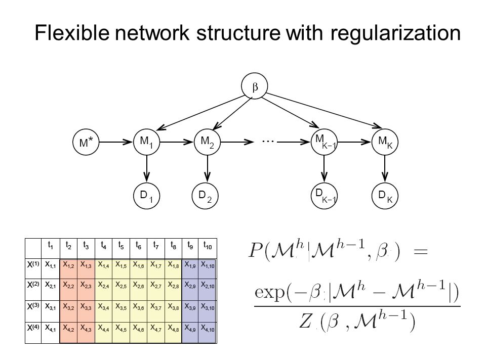
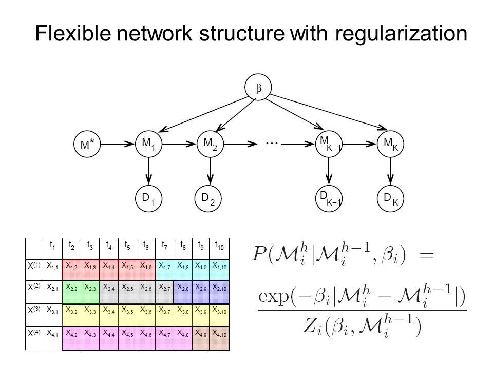
Flexible network structure with regularization

45
ICML 2010

46
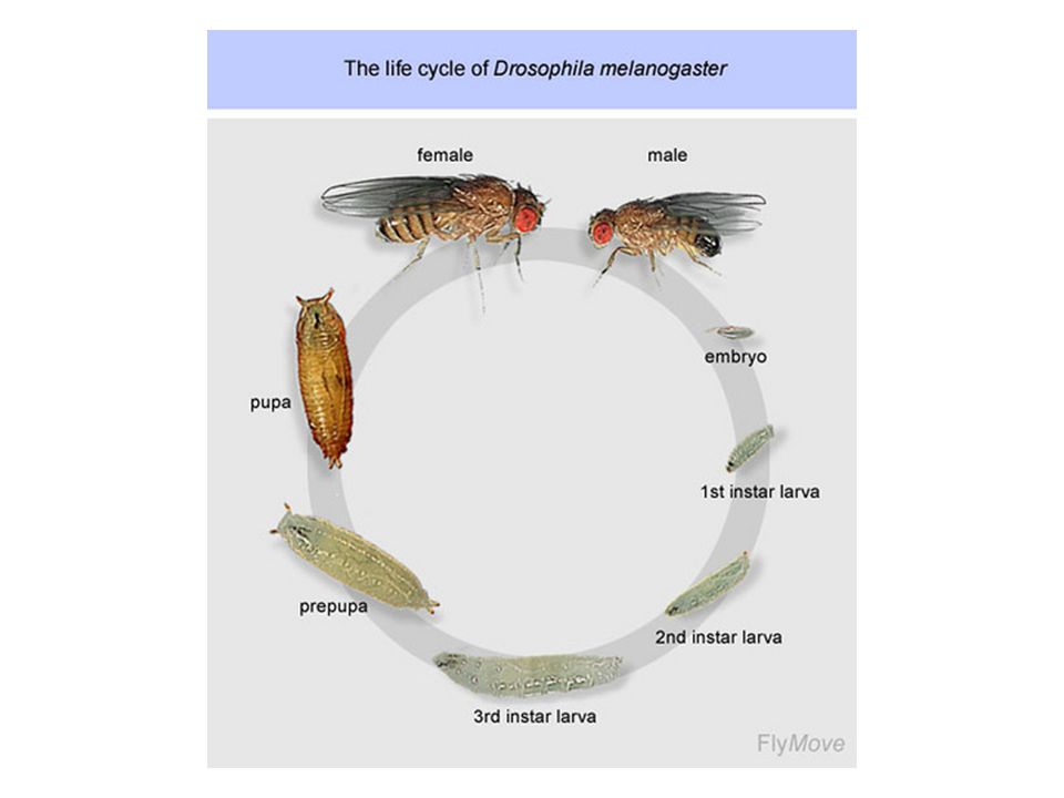
Morphogenesis in Drosophila melanogaster Gene expression measurements over 66 time steps of 4028 genes (Arbeitman et al., Science, 2002). Selection of 11 genes involved in muscle development. Zhao et al. (2006), Bioinformatics 22
, Bioinformatics 22.")
47
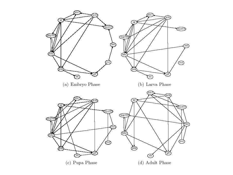
Transition probabilities: flexible structure with regularization Morphogenetic transitions: Embryo larva larva pupa pupa adult

50
Overview Introduction Application to synthetic biology Lessons from DREAM

54
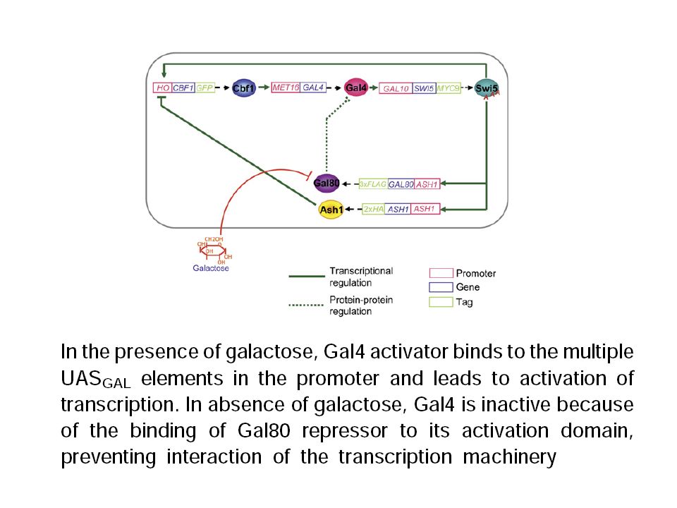
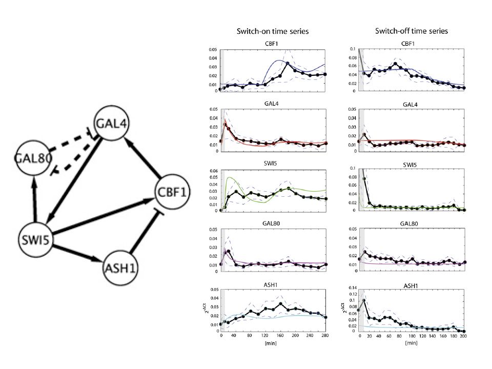
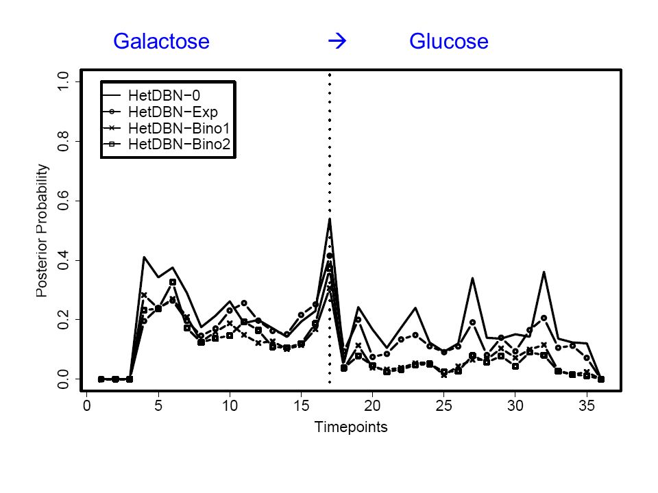
Can we learn the switch Galactose Glucose? Can we learn the network structure?

55
NIPS 2010

56
Node 1 Node i Node p Hierarchical Bayesian model

60
Node 1 Node i Node p Hierarchical Bayesian model

61
Exponential versus binomial prior distribution Exploration of various information sharing options

62
Task 1: Changepoint detection Switch of the carbon source: Galactose Glucose

64
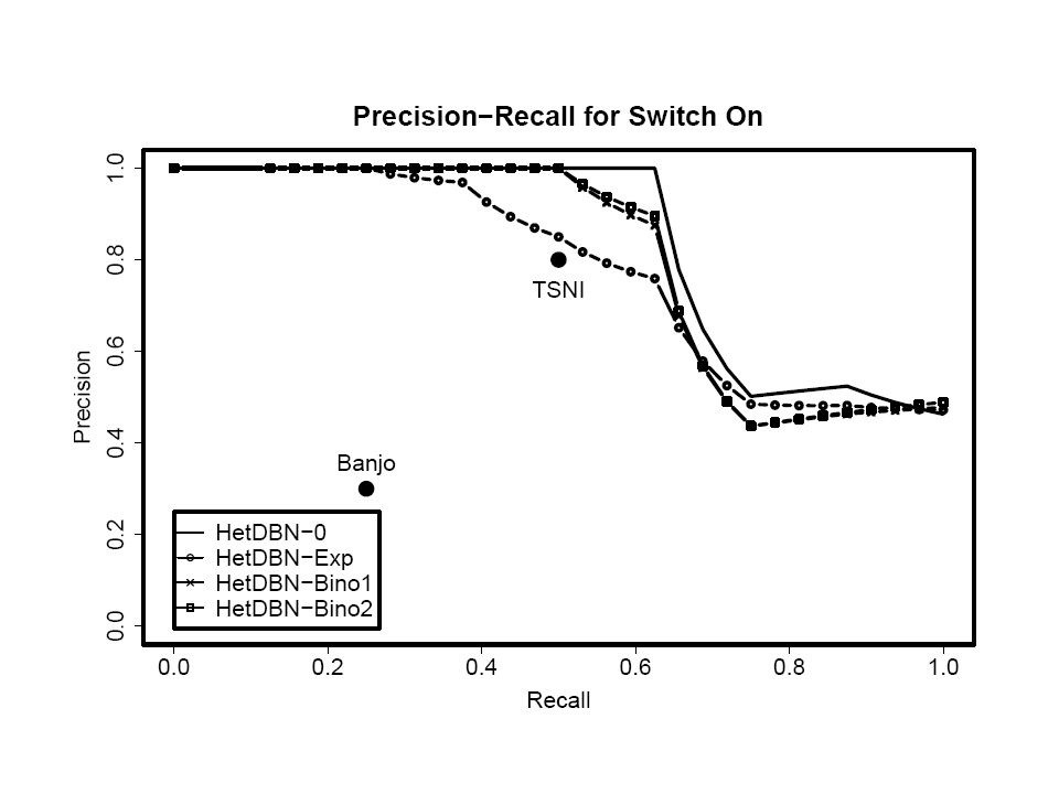
Task 2: Network reconstruction Precision Proportion of identified interactions that are correct Recall Proportion of true interactions that we successfully recovered

65
BANJO: Conventional homogeneous DBN TSNI: Method based on differential equations Inference: optimization, “best” network

67
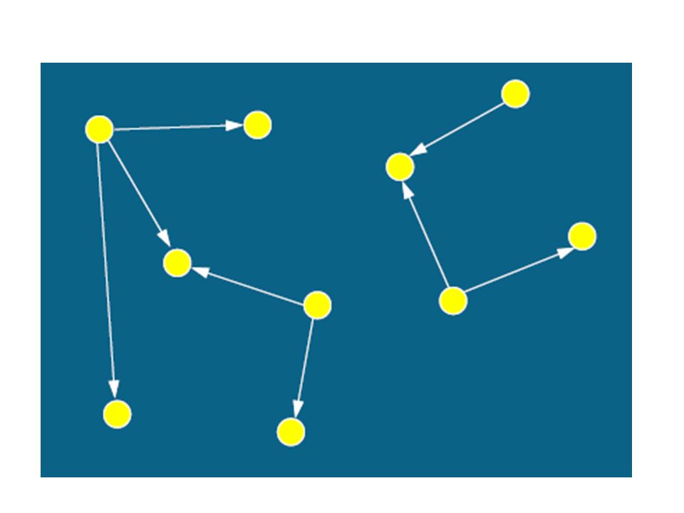
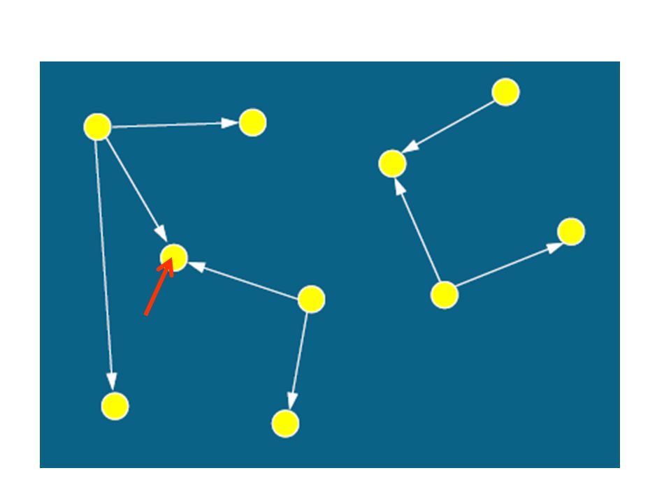
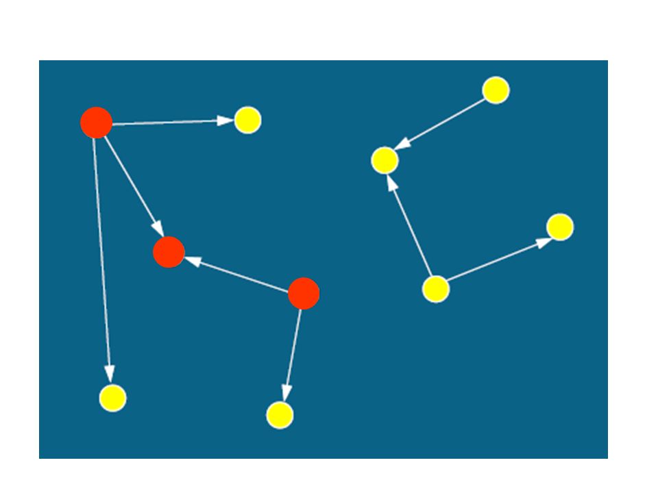
Sample of high-scoring networks

68
Feature extraction, e.g. marginal posterior probabilities of the edges

69
Galactose

70
Glucose

72
PriorCouplingAverage AUC None 0.70 ExponentialHard0.77 BinomialHard0.75 BinomialSoft0.75 Average performance over both phases: Galactose and glucose

73
How are we getting from here …

74
… to there ?!

75
Overview Introduction Application to synthetic biology Lessons from DREAM

76
DREAM: Dialogue for Reverse Engineering Assessments and Methods International network reconstruction competition: June-Sept 2010 Network# Transcription Factors # Genes# Chips Network 1 (in silico) 1951643805 Network 2992810160 Network 33344511805 Network 43335950536
 Network Network Network")
77
Marco Grzegorczyk University of Dortmund Germany Frank Dondelinger BioSS / University of Edinburgh United Kingdom Sophie Lèbre Université de Strasbourg France Our team Andrej Aderhold BioSS / University of St Andrews United Kingdom

78
Our model: Developed for time series Data: Different experimental conditions, perturbations (e.g. ligand injection), interventions (e.g. gene knock-out, overexpression), time points How do we get an ordering of the genes?
, interventions (e.g. gene knock-out, overexpression), time points How do we get an ordering of the genes .")
79
PCA

80
SOM

81
No time series Use 1-dim SOM to get a chip order

82
Ordering of chips changepoint model

83
Problems with MCMC convergence Network# Transcription Factors # Genes# Chips Network 1 (in silico) 1951643805 Network 2992810160 Network 33344511805 Network 43335950536
 Network Network Network")
84
Problems with MCMC convergence Network# Transcription Factors # Genes# Chips Network 1 (in silico) 1951643805 Network 2992810160 Network 33344511805 Network 43335950536 PNAS 2009
 Network Network Network PNAS 2009")
85
[A]= w1[P1] + w2[P2] + w3[P3] + w4[P4] + noise Linear model A P1 P2 P4 P3 w1 w4 w2 w3
![[A]= w1[P1] + w2[P2] + w3[P3] + w4[P4] + noise Linear model A P1 P2 P4 P3 w1 w4 w2 w3](http://images.slideplayer.com/25/7895462/slides/slide_85.jpg "[A]= w1[P1] + w2[P2] + w3[P3] + w4[P4] + noise Linear model A P1 P2 P4 P3 w1 w4 w2 w3")
86
L1 regularized linear regression

87
Problems with MCMC convergence Network# Transcription Factors # Genes# Chips Network 1 (in silico) 1951643805 Network 2992810160 Network 33344511805 Network 43335950536
 Network Network Network")
88
Problems with MCMC convergence Network# Transcription Factors # Genes# Chips Network 1 (in silico) 1951643805 Network 2992810160 Network 33344511805 Network 43335950536
 Network Network Network")
89
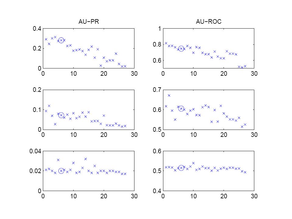
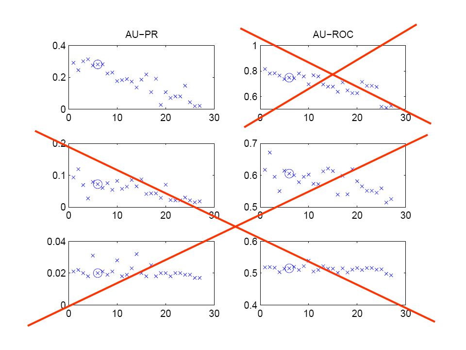
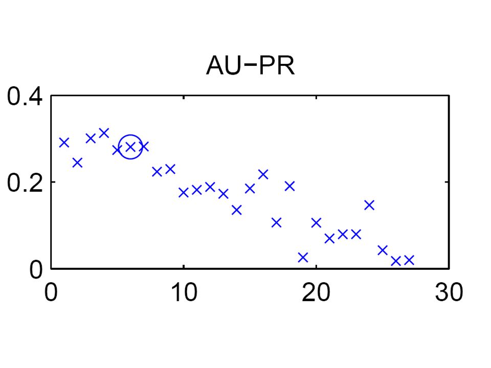
Assessment Participants Had to submit rankings of all interactions Organisers Computed areas under 1)Precision-recall curves 2)ROC curves (plotting sensitivity=recall against specificity)
Precision-recall curves 2)ROC curves (plotting sensitivity=recall against specificity)")
90
Uncertainty about the best network structure Limited number of experimental replications, high noise

91
Sample of high-scoring networks

92
Feature extraction, e.g. marginal posterior probabilities of the edges

93
Sample of high-scoring networks Feature extraction, e.g. marginal posterior probabilities of the edges High-confident edge High-confident non-edge Uncertainty about edges

94
ROC curves True positive rate Sensitivity False positive rate Complementary specificity

95
Definition of metrics Total number of true edges Total number of predicted edges Total number of non-edges Total number of true edges

96
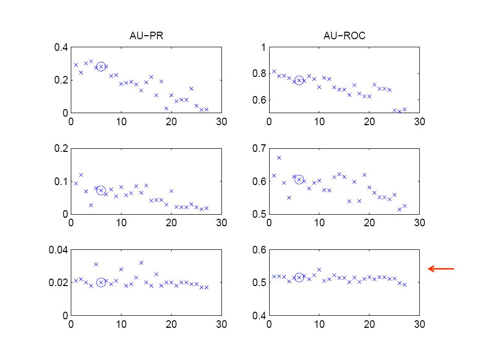
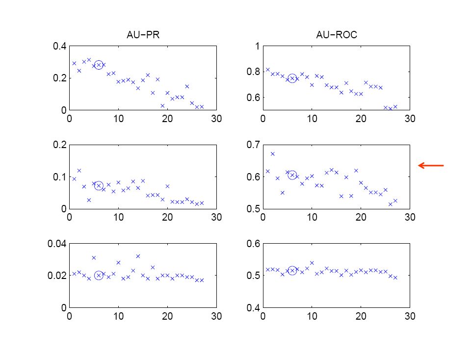
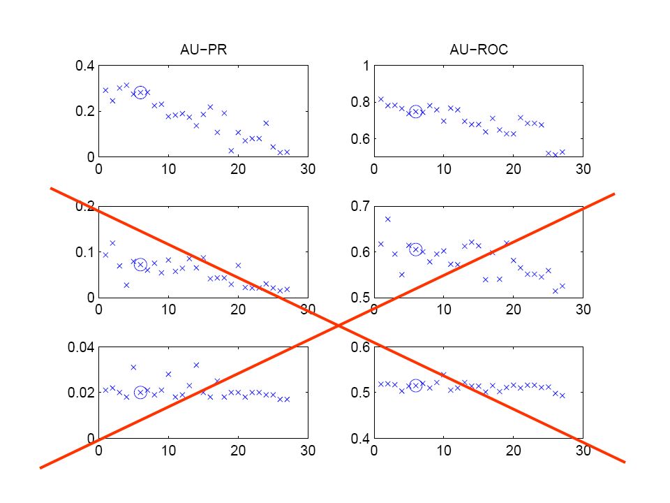
The relation between Precision-Recall (PR) and ROC curves
 and ROC curves")
97
Better performance

98
Assessment Participants Had to submit rankings of all interactions Organisers Computed areas under 1)Precision-recall curves 2)ROC curves (plotting sensitivity=recall against specificity)
Precision-recall curves 2)ROC curves (plotting sensitivity=recall against specificity)")
101
Proportion of recovered true edges Proportion of avoided non-edges AUROC = 0.5

103
Joint work with Wolfgang Lehrach on ab initio prediction of protein interactions AUROC= 0.61,0.67,0.67

105
ICML 2006

106
The relation between Precision-Recall (PR) and ROC curves Better performance
 and ROC curves Better performance")
107
Potential advantage of Precision-Recall (PR) over ROC curves Large number of negative examples (TN+FP) Large change in FP may have a small effect on the false positive rate Large change in FP has a strong effect on the precision Small difference Large difference
 over ROC curves Large number of negative examples (TN+FP) Large change in FP may have a small effect on the false positive rate Large change in FP has a strong effect on the precision Small difference Large difference")
112
Room for improvement: Higher-dimensional changepoint process Perturbations Experimental conditions

Similar presentations


>")


 11/05/07. Methods Linear –PCA (Raychaudhuri et al. 2000) –NIR (Gardner et al. 2003) Nonlinear –Bayesian network (Friedman.>")


