Download presentation
Presentation is loading. Please wait.

1
Uncertainty in Uncertainty

2
Within a factor of 2

3
Impact of noise on precision; applications to GPS data in New Madrid Seismic Zone GIPSY Processing of GPS; central US Short tutorial Estimating the background noise from GPS Using noise to evaluate monument stability Velocities and strain rate estimates Strategy to improve signal to noise

4
GIPSY processing Regional filtering; NA “fixed” http://earthquake.usgs.gov/monitoring/gps/CentralUS/

5
Additional processing Use local sites to remove additional, common-mode translations

6
Standard processing

7
Additional processing

8
Noise Models White Noise

9
Noise Models FLICKER

10
Noise Models Random Walk

11
Noise Models Band Passed filtered; Seasonals

12
Example of GPS noise Random Walk

13
Noise modeling of time series Time, days RMS of [x(t + τ) - x(t)] Red are the data Black are the results of simulations of Flicker and white noise; the average from the simulation and the 95% limits
![Noise modeling of time series Time, days RMS of [x(t + τ) - x(t)] Red are the data Black are the results of simulations of Flicker and white noise; the average from the simulation and the 95% limits](http://images.slideplayer.com/25/7891853/slides/slide_13.jpg "Noise modeling of time series Time, days RMS of [x(t + τ) - x(t)] Red are the data Black are the results of simulations of Flicker and white noise; the average from the simulation and the 95% limits")
14
Noise modeling of time series Comparison between two “end-member” noise models Results suggest that the RW model is more successful than the FL model at the longer periods.

15
Noise modeling of time series Variogram of data compared with 4 different noise models; Either PL or FL+RW models are more successful representing these data.

16
Noise modeling of time series Variogram of data compared with 8 different noise models; Either PL or FL+RW models are most successful representing these data.

17
Sensitivity of rate uncertainty to sampling Flicker noise insensitive to rates > 1 month White noise; sensitive - 1/n^0.5 Random walk insensitive to sampling rate

18
Error in Rate; length of data

19
Random walk becomes marginally detectable at periods > 300 days

20
Error in Rate; length of data Random walk becomes marginally detectable at periods > 300 days But random walk does affect rate errors for periods > 40 days

21
Error in Rate; length of data Random walk becomes marginally detectable at periods > 300 days But random walk does affect rate errors for periods > 40 days 1/T 1. 5 1/T 1/T 0. 5

22
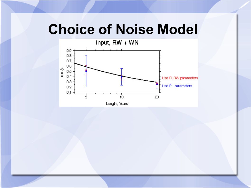
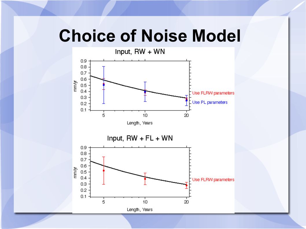
Choice of Noise Model

26
Choice of Noise Model; an extreme example Simulate 20 yrs of data using WN + FL + RW Compute PSD (black) Red is prescribed noise
 Red is prescribed noise")
27
Choice of Noise Model; an extreme example Simulate 20 yrs of data using WN + FL + RW Compute PSD (black) Red is prescribed noise Model as WN + FL + RW
 Red is prescribed noise Model as WN + FL + RW")
28
Choice of Noise Model; an extreme example Simulate 20 yrs of data using WN + FL + RW Compute PSD (black) Red is prescribed noise Model as WN + FL + RW Model as WN + PL
 Red is prescribed noise Model as WN + FL + RW Model as WN + PL")
29
Choice of Noise Model; an extreme example Simulate 20 yrs of data using WN + FL + RW Compute PSD (black) Red is prescribed noise Model as WN + FL + RW Model as WN + PL Same simulation extended to 100 yrs PSD
 Red is prescribed noise Model as WN + FL + RW Model as WN + PL Same simulation extended to 100 yrs PSD")
30
Monument Pictures gode blmm, cnwm, okom ?? arfy/cors arbt/cors

31
Monument comparisons Red – Central US Black – SCIGN

32
Monument comparisons Red – Central US Black – SCIGN Comparison of 2 sites in NMSZ having braced monuments; caution – sites only have 3 years of data; many sites have ~10 years of data

33
Monument comparisons Red – Central US Black – SCIGN Three sites used as regional filter sites with long time-series and excellent stability Classified as “tower” but might not be the same construction used at CORS sites.

34
Braced/CERI Comparison Baseline Length Length= 48.2KM hces – ptgv 1-year of data Braced pair CERI pair Reference G. Mattioli; Aug 2007 NEHRP report# 02JQGR0107

35
Velocities

37
Velocity comparisons

38
Strain Calculation by D. Agnew Eee; detectable RW component of 18 ns/rt(yr) → -2.2+-5.5 ns/yr Enn; RW not significant but, could be 5 ns/rt(yr) → 0.1+-1.6 ns/yr Een; RW not significant but, could be 4 ns/rt(yr) → -1.8+-1.2 ns/yr
 → ns/yr Enn; RW not significant but, could be 5 ns/rt(yr) → ns/yr Een; RW not significant but, could be 4 ns/rt(yr) → ns/yr.")
39
Concluding Remarks Although difficult to quantify, the presence of RW has a significant impact on the precision of the velocity estimates. Long time series will constrain the maximum amplitude of RW noise Long time series, in the presence of RW noise will see a 1/t 0.5 improvement in rate uncertainty. Frequent observations do not improve rate uncertainty but do provide estimates of precision On the other hand, if RW is not justified, then frequent observations provide marginal improvement of rate uncertainty Justification for RW noise comes from long baseline strainmeter data which precisely measures the change in distance between two monuments

40
Items to consider: Short term items – Why does pigt drift east? Install second site at/near pigt Monitor tilt of pigt pier Persistent scatter InSar near pigt Reactivate the Mattioli sites; hces and pgtv Replace antenna at hces (noisy)? Redo USGS solutions to obtain better precision Long term items Campaign/Survey mode GPS Reoccupy existing campaign, GPS sites Additional continuous GPS, where?
. Redo USGS solutions to obtain better precision Long term items Campaign/Survey mode GPS Reoccupy existing campaign, GPS sites Additional continuous GPS, where .")
41
Calais's estimates

42
Compare GIPSY and Calais's GIPSY/USGS GAMIT/Calais

Similar presentations


, Tonie van Dam (U. Luxembourg), Zuheir Altamimi (IGN), Xavier.>")


 of representative samples or strength parameters or slope.>")


 is average of last m observations>")


, Norsang Gelsor 1) and Jens Havskov 2) 1) Jiangsu Road No 36 Lhasa, Tibet, PRC 2) University of Bergen, Department.>")


