Download presentation
Presentation is loading. Please wait.

1
Reinforcement Learning Slides for this part are adapted from those of Dan Klein@UCB And also Alan Fern@ORST

4
Does self learning through simulator. [Infants don’t get to “simulate” the world since they neither have T(.) nor R(.) of their world] Although, once they learn to speak, th Can use their parents as simulators “and what happends if I do this?”
 nor R(.) of their world] Although, once they learn to speak, th Can use their parents as simulators and what happends if I do this .")
5
Objective(s) of Reinforcement Learning Given – your effectors and perceptors Assume full observability of state as well as rewardxx – The world (raw in tooth and claw) – (sometimes) a simulator [so you get ergodicity and can repeat futures] Learn how to perform well – This may involve Learning state values – State rewards have to be learned too; but this is easy Learning action values – (q-function; so we can pick the right action) Learning transition model – (representation; so we can put the rewards and transition using Bellman equations to learn value and policy) Learning policy directly – So we can short circuit and go directly to what is the right thing to do
![Objective(s) of Reinforcement Learning Given – your effectors and perceptors Assume full observability of state as well as rewardxx – The world (raw in tooth and claw) – (sometimes) a simulator [so you get ergodicity and can repeat futures] Learn how to perform well – This may involve Learning state values – State rewards have to be learned too; but this is easy Learning action values – (q-function; so we can pick the right action) Learning transition model – (representation; so we can put the rewards and transition using Bellman equations to learn value and policy) Learning policy directly – So we can short circuit and go directly to what is the right thing to do](http://images.slideplayer.com/25/7870306/slides/slide_5.jpg "Objective(s) of Reinforcement Learning Given – your effectors and perceptors Assume full observability of state as well as rewardxx – The world (raw in tooth and claw) – (sometimes) a simulator [so you get ergodicity and can repeat futures] Learn how to perform well – This may involve Learning state values – State rewards have to be learned too; but this is easy Learning action values – (q-function; so we can pick the right action) Learning transition model – (representation; so we can put the rewards and transition using Bellman equations to learn value and policy) Learning policy directly – So we can short circuit and go directly to what is the right thing to do")
6
Dimensions of Variation of RL Algorithms Model-based vs. Model-free – Model-based Have/learn action models (i.e. transition probabilities) Eg. Approximate DP – Model-free Skip them and directly learn what action to do when (without necessarily finding out the exact model of the action) E.g. Q-learning Passive vs. Active – Passive: Assume the agent is already following a policy (so there is no action choice to be made; it just needs to learn the state values and may be action model) – Active: Need to learn both the optimal policy and the state values (and may be action model)
 Eg. Approximate DP – Model-free Skip them and directly learn what action to do when (without necessarily finding out the exact model of the action) E.g. Q-learning Passive vs. Active – Passive: Assume the agent is already following a policy (so there is no action choice to be made; it just needs to learn the state values and may be action model) – Active: Need to learn both the optimal policy and the state values (and may be action model).")
7
Dimensions of variation (Contd) Extent of Backup Full DP – Adjust value based on values of all the neighbors (as predicted by the transition model) – Can only be done when transition model is present Temporal difference – Adjust value based only on the actual transitions observed Generalization Learn Tabular representations Learn feature-based (factored) representations – Online inductive learning methods..
 Extent of Backup Full DP – Adjust value based on values of all the neighbors (as predicted by the transition model) – Can only be done when transition model is present Temporal difference – Adjust value based only on the actual transitions observed Generalization Learn Tabular representations Learn feature-based (factored) representations – Online inductive learning methods..")
8
When you were a kid, your policy was mostly dictated by your parents (if it is 6AM, wake up and go to school). You however did “learn” to detest Mondays and look for ward to Fridays..

9
(Monte Carlo)
")
10
Inductive Learning over direct estimation States are represented in terms of features The long term cumulative rewards experienced from the states become their labels Do inductive learning (regression) to find the function that maps features to values – This generalizes the experience beyond the specific states we saw
 to find the function that maps features to values – This generalizes the experience beyond the specific states we saw")
11
We are basically doing EMPIRICAL Policy Evaluation! But we know this will be wasteful (since it misses the correlation between values of neibhoring states!) Do DP-based policy evaluation!
 Do DP-based policy evaluation!.")
12
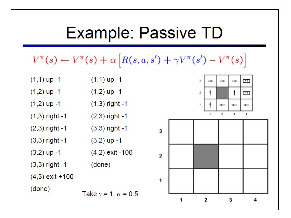
Passive

14
Robustness in the face of Model Uncertainty Suppose you ran through a red light a couple of times, and reached home faster – Should we learn that running through red lights is a good action? General issue with maximum-likelihood learning – If you tossed a coin thrice and it came heads twice, can you say that the probability of heads is 2/3? – General solution: Bayesian Learning Keep a prior on the hypothesis space; and compute posterior given the examples Bayesian Reinforcement Learning – Risk Averse solution Suppose your model is one of K, do the action that is least harmful across the K models

15
Active Model Completeness issue

17
Greedy in the Limit of Infinite Exploration Must try all state-action combinations infinitely often; but must become greedy in the limit

18
9/19

19
(e.g set it to f(1/t) Idea: Keep track of the number of times a state/action pair has been explored; below a threshold, boost the value of that pair (optimism for exploration)
 Idea: Keep track of the number of times a state/action pair has been explored; below a threshold, boost the value of that pair (optimism for exploration)")
20
U+ is set to R+ (max optimistic reward) as long as N(s,a) is below a threshold
 as long as N(s,a) is below a threshold")
21
Model-Free Learning Learn value of a policy (passive) or the best policy (active) without bothering to learn T(.) – Motivation: In some cases, T(.) is too big (e.g. action done from a state can potentially take you to a potentially huge number of states) Rather than wait for T(.) to converge, go directly with experience – Have we seen a model-free RL until now? Monte Carlo (Direct Estimation)
 Rather than wait for T(.) to converge, go directly with experience – Have we seen a model-free RL until now. Monte Carlo (Direct Estimation).")
22
Qn: What if a very unlikely negative (or positive) transition biases the estimate? We already did this for Monte Carlo..

24
Temporal Difference won‘t directly work for Active Learning

29
Dimensions of Variation of RL Algorithms Model-based vs. Model-free – Model-based Have/learn action models (i.e. transition probabilities) Eg. Approximate DP – Model-free Skip them and directly learn what action to do when (without necessarily finding out the exact model of the action) E.g. Q-learning Passive vs. Active – Passive: Assume the agent is already following a policy (so there is no action choice to be made; it just needs to learn the state values and may be action model) – Active: Need to learn both the optimal policy and the state values (and may be action model)
 Eg. Approximate DP – Model-free Skip them and directly learn what action to do when (without necessarily finding out the exact model of the action) E.g. Q-learning Passive vs. Active – Passive: Assume the agent is already following a policy (so there is no action choice to be made; it just needs to learn the state values and may be action model) – Active: Need to learn both the optimal policy and the state values (and may be action model).")
30
Learning/Planning/Acting Model-based vs. Model-Free What you miss in the absence of a model is the ability to “simulate in your mind” You can’t draw an RTDP tree if all you have are Q* values—since Q* tells you what action you should do in a state but wont tell you where that would lead you… --For that latter bit, you need to actually ACT in the world (If you have an external simulator, you can use that in lieu of the world but you still can’t do the RTDP tree in your mind)
.")
31
Dimensions of variation (Contd) Extent of Backup Full DP – Adjust value based on values of all the neighbors (as predicted by the transition model) – Can only be done when transition model is present Temporal difference – Adjust value based only on the actual transitions observed Just the next state Monte-carlo TD( ) Generalization Learn Tabular representations Learn feature-based (factored) representations – Online inductive learning methods..
 Extent of Backup Full DP – Adjust value based on values of all the neighbors (as predicted by the transition model) – Can only be done when transition model is present Temporal difference – Adjust value based only on the actual transitions observed Just the next state Monte-carlo TD( ) Generalization Learn Tabular representations Learn feature-based (factored) representations – Online inductive learning methods..")
32
Relating TD and Monte Carlo (n-step returns) Both Monte Carlo and TD learn from samples (traces) – Monte Carlo waits until the trace hits a sink state, and then (discount) adds all the rewards of the trace – TD on the other hand considers the current state s, and the next experienced state s0 You can think of what TD is doing as “truncating” the experience and summarizing the aggregated reward of the entire trace starting from s0 in terms of the current value estimate of s0 – Why truncate at the very first state s’? How about going from s s0 s1 s2 .. sk and truncate the remaining trace (by assuming that its aggregate reward is just the current value of sk) (sort of like how deep down you go in game trees before applying evaluation function) – In this generalized view, TD corresponds to k=0 and Monte Carlo corresponds to k=infinity
 (sort of like how deep down you go in game trees before applying evaluation function) – In this generalized view, TD corresponds to k=0 and Monte Carlo corresponds to k=infinity.")
33
Averaging over 1..n step returns TD to TD( TD( can be thought of as doing 1,2…k step predictions of the value of the state, and taking their weighted average – Weighting is done in terms of such that – corresponds to TD – corresponds to Monte Carlo Note that the last backup doesn’t have (1- factor… No (1- factor! Reason: After T th state the remaining infinite # states will all have the same aggregated Backup—but each is discounted in. So, we have a 1/(1- factor that Cancels out the (1-

34
SARSA (State-Action-Reward-State-Action) Q-learning is not as fully dependent on the experience as you might think – You are assuming that the best action a’ will be done from s’ (where best action is computed by maxing over Q values) – Why not actually see what action actually got done? SARSA—wait to see what action actually is chosen (no maxing) SARSA is on-policy (it watches the policy) while Q-learning is off- policy (it predicts what action will be done) – SARSA is more realistic and thus better when, let us say, the agent is in a multi-agent world where it is being “lead” from action to action.. E.g. A kid passing by a candy store on the way to school and expecting to stop there, but realizing that his mom controls the steering wheel. – Q-learning is more flexible (it will learn the actual values even when it is being guided by a random policy)
 SARSA is on-policy (it watches the policy) while Q-learning is off- policy (it predicts what action will be done) – SARSA is more realistic and thus better when, let us say, the agent is in a multi-agent world where it is being lead from action to action.. E.g. A kid passing by a candy store on the way to school and expecting to stop there, but realizing that his mom controls the steering wheel. – Q-learning is more flexible (it will learn the actual values even when it is being guided by a random policy).")
35
Full vs. Partial Backups

36
Dimensions of Reinforcement Learning. Monte-carlo tree search

37
Factored Reinforcement Learning after this..

38
10/14 --Factored TD and Q-learning --Policy search (has to be factored..)
")
39
39 Large State Spaces When a problem has a large state space we can not longer represent the V or Q functions as explicit tables Even if we had enough memory – Never enough training data! – Learning takes too long What to do?? [Slides from Alan Fern]

40
40 Function Approximation Never enough training data! – Must generalize what is learned from one situation to other “similar” new situations Idea: – Instead of using large table to represent V or Q, use a parameterized function The number of parameters should be small compared to number of states (generally exponentially fewer parameters) – Learn parameters from experience – When we update the parameters based on observations in one state, then our V or Q estimate will also change for other similar states I.e. the parameterization facilitates generalization of experience
 – Learn parameters from experience – When we update the parameters based on observations in one state, then our V or Q estimate will also change for other similar states I.e. the parameterization facilitates generalization of experience.")
41
41 Linear Function Approximation Define a set of state features f1(s), …, fn(s) – The features are used as our representation of states – States with similar feature values will be considered to be similar A common approximation is to represent V(s) as a weighted sum of the features (i.e. a linear approximation) The approximation accuracy is fundamentally limited by the information provided by the features Can we always define features that allow for a perfect linear approximation? – Yes. Assign each state an indicator feature. (I.e. i’th feature is 1 iff i’th state is present and i represents value of i’th state) – Of course this requires far to many features and gives no generalization.
 The approximation accuracy is fundamentally limited by the information provided by the features Can we always define features that allow for a perfect linear approximation. – Yes. Assign each state an indicator feature. (I.e. i’th feature is 1 iff i’th state is present and i represents value of i’th state) – Of course this requires far to many features and gives no generalization..")
42
42 Example Consider grid problem with no obstacles, deterministic actions U/D/L/R (49 states) Features for state s=(x,y): f1(s)=x, f2(s)=y (just 2 features) V(s) = 0 + 1 x + 2 y Is there a good linear approximation? – Yes. – 0 =10, 1 = -1, 2 = -1 – (note upper right is origin) V(s) = 10 - x - y subtracts Manhattan dist. from goal reward 10 0 0 6 6
 V(s) = 10 - x - y subtracts Manhattan dist. from goal reward")
43
43 But What If We Change Reward … V(s) = 0 + 1 x + 2 y Is there a good linear approximation? – No. 10 0 0

44
44 But What If… V(s) = 0 + 1 x + 2 y 10 + 3 z Include new feature z z= |3-x| + |3-y| z is dist. to goal location Does this allow a good linear approx? 0 =10, 1 = 2 = 0, 0 = -1 0 0 3 3 Feature Engineering….

47
47 Linear Function Approximation Define a set of features f1(s), …, fn(s) – The features are used as our representation of states – States with similar feature values will be treated similarly – More complex functions require more complex features Our goal is to learn good parameter values (i.e. feature weights) that approximate the value function well – How can we do this? – Use TD-based RL and somehow update parameters based on each experience.
 that approximate the value function well – How can we do this. – Use TD-based RL and somehow update parameters based on each experience..")
48
48 TD-based RL for Linear Approximators 1.Start with initial parameter values 2.Take action according to an explore/exploit policy (should converge to greedy policy, i.e. GLIE) 3.Update estimated model 4.Perform TD update for each parameter 5.Goto 2 What is a “TD update” for a parameter?
 3.Update estimated model 4.Perform TD update for each parameter 5.Goto 2 What is a TD update for a parameter .")
49
49 Aside: Gradient Descent Given a function f( 1,…, n ) of n real values = ( 1,…, n ) suppose we want to minimize f with respect to A common approach to doing this is gradient descent The gradient of f at point , denoted by f( ), is an n-dimensional vector that points in the direction where f increases most steeply at point Vector calculus tells us that f( ) is just a vector of partial derivatives where can decrease f by moving in negative gradient direction
 of n real values = ( 1,…, n ) suppose we want to minimize f with respect to A common approach to doing this is gradient descent The gradient of f at point , denoted by f( ), is an n-dimensional vector that points in the direction where f increases most steeply at point Vector calculus tells us that f( ) is just a vector of partial derivatives where can decrease f by moving in negative gradient direction")
50
50 Aside: Gradient Descent for Squared Error Suppose that we have a sequence of states and target values for each state – E.g. produced by the TD-based RL loop Our goal is to minimize the sum of squared errors between our estimated function and each target value: After seeing j’th state the gradient descent rule tells us that we can decrease error by updating parameters by: squared error of example j our estimated value for j’th state learning rate target value for j’th state

51
51 Aside: continued For a linear approximation function: Thus the update becomes: For linear functions this update is guaranteed to converge to best approximation for suitable learning rate schedule depends on form of approximator

52
52 TD-based RL for Linear Approximators 1.Start with initial parameter values 2.Take action according to an explore/exploit policy (should converge to greedy policy, i.e. GLIE) Transition from s to s’ 3.Update estimated model 4.Perform TD update for each parameter 5.Goto 2 What should we use for “target value” v(s)? Use the TD prediction based on the next state s’ this is the same as previous TD method only with approximation
 Transition from s to s’ 3.Update estimated model 4.Perform TD update for each parameter 5.Goto 2 What should we use for target value v(s). Use the TD prediction based on the next state s’ this is the same as previous TD method only with approximation.")
53
53 TD-based RL for Linear Approximators 1.Start with initial parameter values 2.Take action according to an explore/exploit policy (should converge to greedy policy, i.e. GLIE) 3.Update estimated model 4.Perform TD update for each parameter 5.Goto 2 Step 2 requires a model to select greedy action For applications such as Backgammon it is easy to get a simulation-based model For others it is difficult to get a good model But we can do the same thing for model-free Q-learning
 3.Update estimated model 4.Perform TD update for each parameter 5.Goto 2 Step 2 requires a model to select greedy action For applications such as Backgammon it is easy to get a simulation-based model For others it is difficult to get a good model But we can do the same thing for model-free Q-learning.")
54
54 Q-learning with Linear Approximators 1.Start with initial parameter values 2.Take action a according to an explore/exploit policy (should converge to greedy policy, i.e. GLIE) transitioning from s to s’ 3.Perform TD update for each parameter 4.Goto 2 For both Q and V, these algorithms converge to the closest linear approximation to optimal Q or V. Features are a function of states and actions.
 transitioning from s to s’ 3.Perform TD update for each parameter 4.Goto 2 For both Q and V, these algorithms converge to the closest linear approximation to optimal Q or V. Features are a function of states and actions..")
55
55 Example: Tactical Battles in Wargus Wargus is real-time strategy (RTS) game – Tactical battles are a key aspect of the game RL Task: learn a policy to control n friendly agents in a battle against m enemy agents – Policy should be applicable to tasks with different sets and numbers of agents 5 vs. 5 10 vs. 10

62
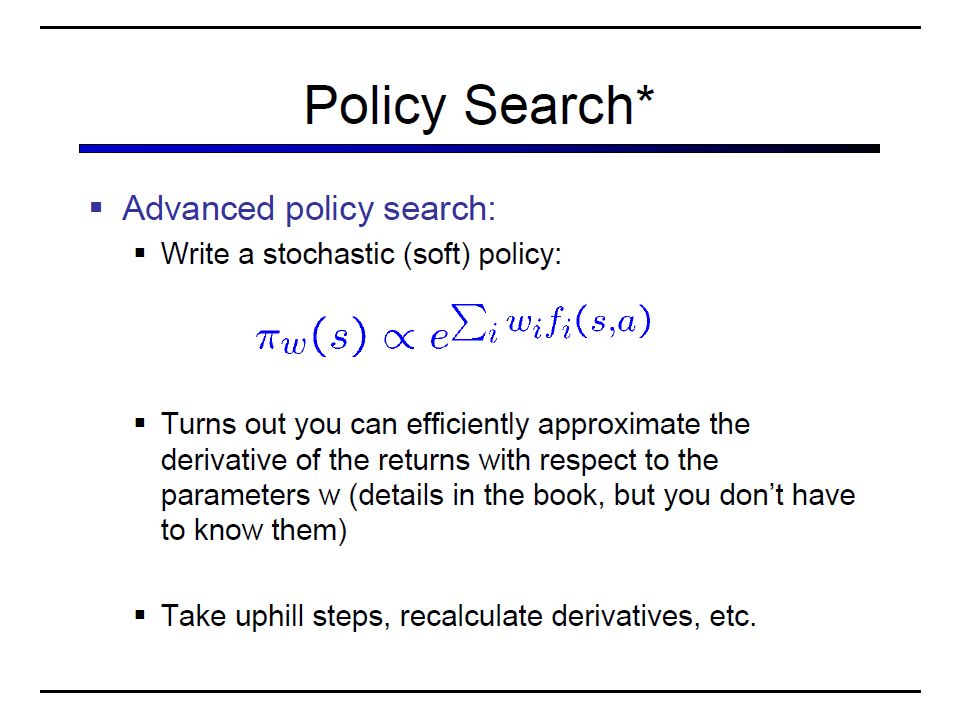
62 Policy Gradient Ascent Let ( ) be the expected value of policy . – ( ) is just the expected discounted total reward for a trajectory of . – For simplicity assume each trajectory starts at a single initial state. Our objective is to find a that maximizes ( ) Policy gradient ascent tells us to iteratively update parameters via: Problem: ( ) is generally very complex and it is rare that we can compute a closed form for the gradient of ( ). We will instead estimate the gradient based on experience
 is just the expected discounted total reward for a trajectory of . – For simplicity assume each trajectory starts at a single initial state. Our objective is to find a that maximizes ( ) Policy gradient ascent tells us to iteratively update parameters via: Problem: ( ) is generally very complex and it is rare that we can compute a closed form for the gradient of ( ). We will instead estimate the gradient based on experience.")
63
63 Gradient Estimation Concern: Computing or estimating the gradient of discontinuous functions can be problematic. For our example parametric policy is ( ) continuous? No. – There are values of where arbitrarily small changes, cause the policy to change. – Since different policies can have different values this means that changing can cause discontinuous jump of ( ).
 continuous. No. – There are values of where arbitrarily small changes, cause the policy to change. – Since different policies can have different values this means that changing can cause discontinuous jump of ( )..")
64
64 Example: Discontinous ( ) Consider a problem with initial state s and two actions a1 and a2 – a1 leads to a very large terminal reward R1 – a2 leads to a very small terminal reward R2 Fixing 2 to a constant we can plot the ranking assigned to each action by Q and the corresponding value ( ) 11 11 ()() R1 R2 Discontinuity in ( ) when ordering of a1 and a2 change
 Consider a problem with initial state s and two actions a1 and a2 – a1 leads to a very large terminal reward R1 – a2 leads to a very small terminal reward R2 Fixing 2 to a constant we can plot the ranking assigned to each action by Q and the corresponding value ( ) 11 11 ()() R1 R2 Discontinuity in ( ) when ordering of a1 and a2 change")
65
65 Probabilistic Policies We would like to avoid policies that drastically change with small parameter changes, leading to discontinuities A probabilistic policy takes a state as input and returns a distribution over actions – Given a state s (s,a) returns the probability that selects action a in s Note that ( ) is still well defined for probabilistic policies – Now uncertainty of trajectories comes from environment and policy – Importantly if (s,a) is continuous relative to changing then ( ) is also continuous relative to changing A common form for probabilistic policies is the softmax function or Boltzmann exploration function Aka Mixed Policy (not needed for Optimality…)
 returns the probability that selects action a in s Note that ( ) is still well defined for probabilistic policies – Now uncertainty of trajectories comes from environment and policy – Importantly if (s,a) is continuous relative to changing then ( ) is also continuous relative to changing A common form for probabilistic policies is the softmax function or Boltzmann exploration function Aka Mixed Policy (not needed for Optimality…)")
66
66 Empirical Gradient Estimation Our first approach to estimating ( ) is to simply compute empirical gradient estimates Recall that = ( 1,…, n) and so we can compute the gradient by empirically estimating each partial derivative So for small we can estimate the partial derivatives by This requires estimating n+1 values:
 is to simply compute empirical gradient estimates Recall that = ( 1,…, n) and so we can compute the gradient by empirically estimating each partial derivative So for small we can estimate the partial derivatives by This requires estimating n+1 values:")
67
67 Empirical Gradient Estimation How do we estimate the quantities For each set of parameters, simply execute the policy for N trials/episodes and average the values achieved across the trials This requires a total of N(n+1) episodes to get gradient estimate – For stochastic environments and policies the value of N must be relatively large to get good estimates of the true value – Often we want to use a relatively large number of parameters – Often it is expensive to run episodes of the policy So while this can work well in many situations, it is often not a practical approach computationally Better approaches try to use the fact that the stochastic policy is differentiable. – Can get the gradient by just running the current policy multiple times Doable without permanent damage if there is a simulator

68
68 Applications of Policy Gradient Search Policy gradient techniques have been used to create controllers for difficult helicopter maneuvers For example, inverted helicopter flight. A planner called FPG also “won” the 2006 International Planning Competition – If you don’t count FF-Replan

69
Slides beyond this not discussed

71
71 Policy Gradient Recap When policies have much simpler representations than the corresponding value functions, direct search in policy space can be a good idea – Allows us to design complex parametric controllers and optimize details of parameter settings For baseline algorithm the gradient estimates are unbiased (i.e. they will converge to the right value) but have high variance – Can require a large N to get reliable estimates OLPOMDP offers can trade-off bias and variance via the discount parameter [Baxter & Bartlett, 2000] Can be prone to finding local maxima – Many ways of dealing with this, e.g. random restarts.
 but have high variance – Can require a large N to get reliable estimates OLPOMDP offers can trade-off bias and variance via the discount parameter [Baxter & Bartlett, 2000] Can be prone to finding local maxima – Many ways of dealing with this, e.g. random restarts..")
72
72 Gradient Estimation: Single Step Problems For stochastic policies it is possible to estimate ( ) directly from trajectories of just the current policy – Idea: take advantage of the fact that we know the functional form of the policy First consider the simplified case where all trials have length 1 – For simplicity assume each trajectory starts at a single initial state and reward only depends on action choice – ( ) is just the expected reward of action selected by . where s 0 is the initial state and R(a) is reward of action a The gradient of this becomes How can we estimate this by just observing the execution of ?
 is reward of action a The gradient of this becomes How can we estimate this by just observing the execution of .")
73
73 Rewriting The gradient is just the expected value of g(s 0,a)R(a) over execution trials of – Can estimate by executing for N trials and averaging samples a j is action selected by policy on j’th episode – Only requires executing for a number of trials that need not depend on the number of parameters can get closed form g(s 0,a) Gradient Estimation: Single Step Problems
R(a) over execution trials of – Can estimate by executing for N trials and averaging samples a j is action selected by policy on j’th episode – Only requires executing for a number of trials that need not depend on the number of parameters can get closed form g(s 0,a) Gradient Estimation: Single Step Problems")
74
74 Gradient Estimation: General Case So for the case of a length 1 trajectories we got: For the general case where trajectories have length greater than one and reward depends on state we can do some work and get: s jt is t’th state of j’th episode, a jt is t’th action of epidode j The derivation of this is straightforward but messy. Observed total reward in trajectory j from step t to end length of trajectory j # of trajectories of current policy

75
75 How to interpret gradient expression? So the overall gradient is a reward weighted combination of individual gradient directions – For large R j (s j, t ) will increase probability of a j, t in s j, t – For negative R j (s j, t ) will decrease probability of a j, t in s j, t Intuitively this increases probability of taking actions that typically are followed by good reward sequences Direction to move parameters in order to increase the probability that policy selects a jt in state s jt Total reward observed after taking a jt in state s jt
 will increase probability of a j, t in s j, t – For negative R j (s j, t ) will decrease probability of a j, t in s j, t Intuitively this increases probability of taking actions that typically are followed by good reward sequences Direction to move parameters in order to increase the probability that policy selects a jt in state s jt Total reward observed after taking a jt in state s jt.")
76
76 Basic Policy Gradient Algorithm Repeat until stopping condition 1.Execute for N trajectories while storing the state, action, reward sequences One disadvantage of this approach is the small number of updates per amount of experience – Also requires a notion of trajectory rather than an infinite sequence of experience Online policy gradient algorithms perform updates after each step in environment (often learn faster)
")
77
Online Policy Gradient (OLPOMDP) Repeat forever 1.Observe state s 2.Draw action a according to distribution (s) 3.Execute a and observe reward r 4. ;; discounted sum of ;; gradient directions 5. Performs policy update at each time step and executes indefinitely – This is the OLPOMDP algorithm [Baxter & Bartlett, 2000]

78
Interpretation Repeat forever 1.Observe state s 2.Draw action a according to distribution (s) 3.Execute a and observe reward r 4. ;; discounted sum of ;; gradient directions 5. Step 4 computes an “eligibility trace” e – Discounted sum of gradients over previous state-action pairs – Points in direction of parameter space that increases probability of taking more recent actions in more recent states For positive rewards step 5 will increase probability of recent actions and decrease for negative rewards.

79
79 Computing the Gradient of Policy Both algorithms require computation of For the Boltzmann distribution with linear approximation we have: where Here the partial derivatives needed for g(s,a) are:
 are:")
Similar presentations


 Tue, March 21, 2014.>")


![Ai in game programming it university of copenhagen Reinforcement Learning [Outro] Marco Loog.](/13/4141175/big_thumb.jpg "Ai in game programming it university of copenhagen Reinforcement Learning [Outro] Marco Loog.>")


>")

 Learning –a combination of DP and MC methods updates estimates based on.>")


