1. Modeling Real-World Data
9-6
Modeling Real-World Data
Warm Up
Lesson Presentation
Lesson Quiz
Holt Algebra 2

2. Warm Up quadratic: y ≈ 2.13x2 – 2x + 6.12
1. Use a calculator to perform quadratic and exponential regressions on the following data. x 3 5 8 13 y 19 50
126
340
quadratic: y ≈ 2.13x2 – 2x
exponential: y ≈ 10.57(1.32)x

3. Objectives Apply functions to problem situations.
Use mathematical models to make predictions.

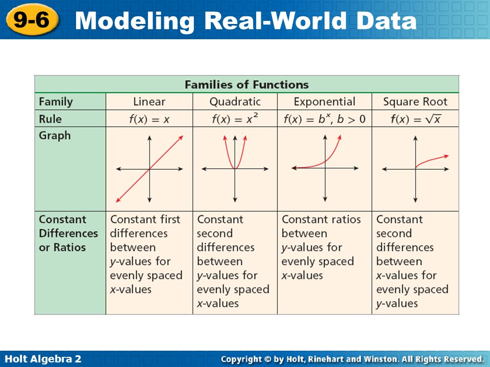
4. Much of the data that you encounter in the real world may form a pattern. Many times the pattern of the data can be modeled by one of the functions you have studied. You can then use the functions to analyze trends and make predictions. Recall some of the parent functions that you have studied so far.

6. Because the square-root function is the inverse of the quadratic function, the constant differences for x- and y-values are switched.
Helpful Hint

7. Example 1A: Identifying Models by Using Constant Differences or Ratios
Use constant differences or ratios to determine which parent function would best model the given data set.
Time (yr) 5 10 15 20 25
Height (in.) 58 93
128
163
198
Notice that the time data are evenly spaced. Check the first differences between the heights to see if the data set is linear.

8. Example 1A Continued
Height (in.) 58 93
128
163
198
First differences
Because the first differences are a constant 35, a linear model will best model the data.

9. Example 1B: Identifying Models by Using Constant Differences or Ratios
Time (yr) 4 8 12 16 20
Population
10,000
9,600
9,216
8,847
8,493
Notice that the time data are evenly spaced. Check the first differences between the populations.
Population
10,000
9,600
9,216
8,847
8,493
First differences – –384 – –354
Second differences

10. Example 1B Continued
Neither the first nor second differences are constant. Check ratios between the volumes.
9216
9600
8847
= 0.96,
10,000
≈ 0.96,
and ≈ 0.96.
8493
8847

11. Example 1B Continued
Because the ratios between the values of the dependent variable are constant, an exponential function would best model the data.
Check A scatter plot reveals a shape similar to an exponential decay function.

12. Example 1C: Identifying Models by Using Constant Differences or Ratios
Time (s) 1 2 3 4 5
Height (m)
132
165
154 99
Notice that the time data are evenly spaced. Check the first differences between the heights.
Height (m)
132
165
154 99
First differences – – –99
Second differences – – –44

13. Example 1C Continued
Because the second differences of the dependent variables are constant when the independent variables are evenly spaced, a quadratic function will best model the data.
Check A scatter reveals a shape similar to a quadratic parent function f(x) = x2.

14. Check It Out! Example 1a
Use constant differences or ratios to determine which parent function would best model the given data set. x 12 48
108
192
300 y 10 20 30 40 50
Notice that the data for the y-values are evenly spaced. Check the first differences between the x-values.

15. Check It Out! Example 1a Continued12 48
108
192
300
First differences
Second differences
Because the second differences of the independent variable are constant when the dependent variables are evenly spaced, a square-root function will best model the data.

16. Check It Out! Example 1b x 21 22 23 24 y
243
324
432
576
Notice that x-values are evenly spaced. Check the differences between the y-values. y
243
324
432
576
First differences
Second differences

17. Check It Out! Example 1b Continued
Neither the first nor second differences are constant. Check ratios between the values.
324
243
≈ 1.33, and
≈ 1.33,
≈ 1.33
432
576

18. Check It Out! Example 1b Continued
Because the ratios between the values of the dependent variable are constant, an exponential function would best model the data.
Check A scatter reveals a shape similar to an exponential decay function.

19. To display the correlation coefficient r on some calculators, you must turn on the diagnostic mode.
Press , and choose DiagnosticOn.
Helpful Hint

20. Example 2: Economic Application
A printing company prints advertising flyers and tracks its profits. Write a function that models the given data.
Flyers Printed
100
200
300
400
500
600
Profit ($) 10 70
175
312
720
Step 1 Make a scatter plot of the data. The data appear to form a quadratic or exponential pattern.

21. Example 2 Continued
Step 1 Analyze differences.
Profit ($) 10 70
175
312
500
720
First differences
Second differences
Because the second differences of the dependent variable are close to constant when the independent variables are evenly spaced, a quadratic function will best model the data.

22. Example 2 Continued
Step 3 Use your graphing calculator to perform a quadratic regression.
A quadratic function that models the data is
f(x) = 0.002x x – The correlation r is very close to 1, which indicates a good fit.

23. Check It Out! Example 2
Write a function that models the given data. x 12 14 16 18 20 22 24 y
110
141
176
215
258
305
356
Step 1 Make a scatter plot of the data. The data appear to form a quadratic or exponential pattern.

24. Check It Out! Example 2 Continued
Step 1 Analyze differences. y
110
141
176
215
258
305
356
First differences
Second differences
Because the second differences of the dependent variable are constant when the independent variables are evenly spaced, a quadratic function will best model the data.

25. Check It Out! Example 2 Continued
Step 3 Use your graphing calculator to perform a quadratic regression.
A quadratic function that models the data is f(x) = 0.5x x + 8. The correlation r is 1, which indicates a good fit.

26. When data are not ordered or evenly spaced, you may to have to try several models to determine which best approximates the data. Graphing calculators often indicate the value of the coefficient of determination, indicated by r2 or R2. The closer the coefficient is to 1, the better the model approximates the data.

27. Example 3: Application
The data shows the population of a small town since Using 1990 as a reference year, write a function that models the data.
Year
1990
1993
1997
2000
2002
2005
2006
Population
400
490
642
787
901
1104
1181
The data are not evenly spaced, so you cannot analyze differences or ratios.

28. • • • • • • • Example 3 Continued
Population
year
1990
2006
1997
2002
2005
1993
400
800
1200
2000 •
Create a scatter plot of the data. Use 1990 as year 0. The data appear to be quadratic, cubic or exponential. • • • • • •

29. Example 3 Continued
Use the calculator to perform each type of regression.
Compare the value of r2. The exponential model seems to be the best fit. The function f(x) ≈ (1.07)x models the data.

30. Write a function that models the data.
Check It Out! Example 3
Write a function that models the data.
Fertilizer/Acre (lb) 11 14 25 31 40 50
Yield/Acre (bushels)
245
302
480
557
645
705
The data are not evenly spaced, so you cannot analyze differences or ratios.

31. Check It Out! Example 3 Continued
Create a scatter plot of the data. The data appear to be quadratic, cubic or exponential.

32. Check It Out! Example 3 Continued
Use the calculator to perform each type of regression.
Compare the value of r2. The cubic model seems to be the best fit. The function f(x) ≈ –9.3x3 –0.2x x

33. 2. Write a function that models the given data.
Lesson Quiz
1. Use finite differences or ratios to determine which parent function would best model the given data set, and write a function that models the data.
Length (ft) 5 10 15 20 25
Cost ($)
102.50
290.00
602.50
quadratic; C(l) = 2.5x2 + 40
2. Write a function that models the given data.
Time (min) 2 4 6 8 10
Volume (cm2)
1.2
3.9
15.7
64.2
256.5
1023.8
f(x) = 1.085(1.977)x