1. Class 4 Simple Linear Regression

2. Regression Analysis Reality is thought to behave in a manner which may be simulated (predicted) to an acceptable degree of accuracy by a simplified mathematical model. Statistical models (which include regression) permit some degree of random error, because some variable of interest cannot be duplicated under seemingly identical conditions.

3. An Example We would like to predict test scores on an academic test. Ten such scores are shown below: A possible model of test scores: A test score, y, is obtained by taking the average test score, , and adding a random value, , to it. 65 73 73 75 81 87 92 96 98 100 y =  + 

4. Example (cont.) How might we estimate  ? How do we tell if our model is useful?

5. Improving the Model We would have a more useful model if we could remove (explain) some of the variability that we see in the data. Perhaps there exists other factors that cause variability in the test score. Can you think of some?

6. Improving the Model (cont.) Here is the data including the hours of study.

7. Improving the Model (cont.) We have the same problem: Select the best line that minimizes the (squared) distance of the data points to the line. This line is referred to as the least square line. Our model now looks like Our estimated or fitted line will be called

8. Another view of the Model This (and all linear regression) model(s) can be expressed as y = E(y) + . So in our model, E(y) =  0 +  1 x, that is, the mean test score falls on a straight line as a function of hours of study. The random error term, , is assumed to have a normal distribution with mean 0 and variance  2. Our ability to effectively use the model depends on this variation.

9. Analysis of Variance It turns out that the variation displayed by the variable y, referred to as the total sum of squares (SST), can be broken into two pieces: The part caused by the variable x, called the regression sum of squares (SSR), The part left over (the distance from the data points to the regression line), called the sum of squared errors or residual sum of squares (SSE). SST = SSR + SSE

10. Getting it done with EXCEL Select tools/data analysis/regression. r, correlation r 2 = SSR/SST s, the square root of s 2, our estimate of  2 r a 2 = 1 - (1-r 2 )[(n-1)/(n-p-1)]

11. Getting it done with EXCEL SSR SSE SST Actual sums of squares Sums of squares divided by degrees of freedom MSR MSE, also s 2 MSR/MSE p-value For example,

12. Getting it done with EXCEL Least square estimates Standard deviation of our estimate t-test for the hypothesis that the coefficient (  ) is 0 The important part: the p-value for the t-test Confidence Intervals for our estimates b0b0 b1b1

13. Hypothesis Testing The F-test tests to see if all of the coefficients of the independent variables are zero. For our model: The t-test tests to see if each coefficient of an independent variables is zero.

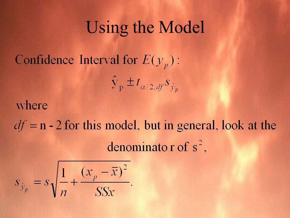
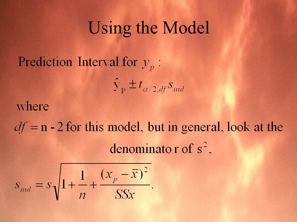
14. Using the Model The model has two basic purposes: (1) It can be used to provide partial confirmation of the theory that a particular factor is, indeed, influencing the response variable, y. (2) It can be used to estimate the mean, E(y), and predict an actual value of y. Under the function wizard, select forecast(new_x, known_y, known_x).

15. Confidence interval can be generated (page 555 for more discussion). Let Using the Model

18. EXCEL does not provide an automatic calculation for confidence and prediction intervals The authors have included a macro in the spreadsheet called PredInt.xls on your data disk. Simply open the file and follow the instructions! Using the Model

19. A Note on Correlation Many people prefer to perform a correlational analysis before they build regression models. In EXCEL this can be accomplished in two ways: Under the function wizard, use correl(array1,array2) to find the correlation between two variables. Under tools/data analysis/correlation to determine the correlation between several variables.

20. Correlation (cont.) What correlation does: Provides an easy measure to determine if two variables have a linear relationship. Positive correlation implies if one variable goes up, the other also tends to go up. Negative correlation implies if one variable goes up, the other tends to go down. What correlation does not do: There is no implication of cause and effect. There may exist some lurking factor that produces the behavior being witnessed.