1. Final Exam Schedule – Fall, 2014 11:00 ClassThursday, December 1110:30 – 12:30 2:00 ClassThursday, December 111:00 – 3:00 3:30 ClassTuesday, December 93:30 – 5:30

2. YearU.S. Population in millions 1950152.3 1960180.7 1970205.1 1980227.7 1990249.9 The table at the right shows the census population of the United States in various years. 1.Find a power model for the data. 2.Graph the data and the power model on your calculator. Warm-up

3. YearU.S. Population in millions 1950152.3 1960180.7 1970205.1 1980227.7 1990249.9 The table at the right shows the census population of the United States in various years. 1.Find a power model for the data. 2.Graph the data and the power model on your calculator. Warm-up x = years since 1900

4. YearU.S. Population in millions 1950152.3 1960180.7 1970205.1 1980227.7 1990249.9 The table at the right shows the census population of the United States in various years. 1.Find a power model for the data. 2.Graph the data and the power model on your calculator. Warm-up x = years since 1940

5. YearU.S. Population in millions 1950152.3 1960180.7 1970205.1 1980227.7 1990249.9 The table at the right shows the census population of the United States in various years. 1.Find a power model for the data. 2.Graph the data and the power model on your calculator. Warm-up x = years

6. Homework Solutions Section 5.2

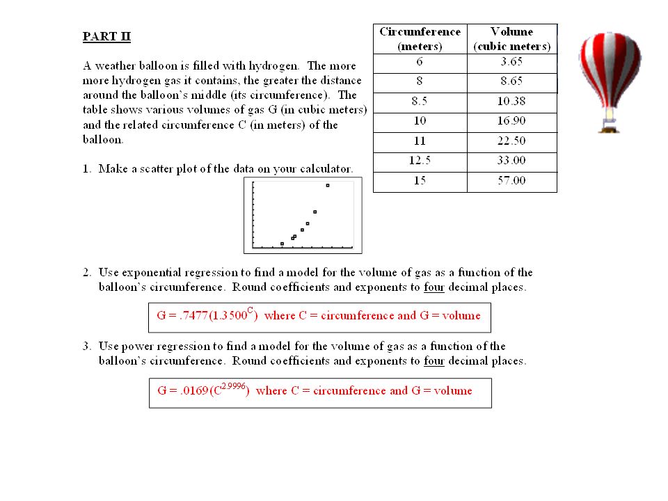
8. The power model is better because it more closely fits the data. The exponential model is rising more quickly than the power model and will predict much too large values for volume of gas when the circumference gets larger. Also the power model’s correlation coefficient r is closer to 1.

9. The power model is better because it more closely fits the data. The exponential model is rising very quickly and will predict much too large values for volume of gas when the circumference gets larger. Also the power model’s correlation coefficient r is closer to 1. The power model is better because it more closely fits the data. The exponential model is rising more quickly than the power model and will predict much too large values for volume of gas when the circumference gets larger. Also the power model’s correlation coefficient r is closer to 1.

10. Composite Functions Given functions f(x) and g(x), the composite of f and g, denoted g(f(x)) or g f, is the function obtained by taking the output of function f and using it as the input of function g. o

11. f(x) = 3x + 5 g(x) = 2x – 4 f(9) = 32 g( ) = 60 g(f( 9 )) = 60 Begin with f(x) using x = 9 What is g(f(9))?

12. f(x) = x 2 – 2x g(x) = 3x f(7) = 35 g( ) Another Example = 105 g(f( 7 )) = 105 Begin with f(x) using x = 7 What is g(f(7))?

13. g(f(x)) is a composite function. g(f(x)) is the composite of f and g. Some examples: If f(x) = 3x + 5 and g(x) = 2x – 4, find: 1.g(f(4)) 2.f(g( – 3)) 3.g(f( )) 4.g(f(0)) = 30 = – 25 = 9 = 6 g(f(17)) g(f(-8)) g(f(52.6)) g(f( )) g(f(105)) g(f(-14.9)) What if you were now asked to find:

14. f(x) = 3x + 5 g(x) = 2x – 4 = 6x + 6 f(x) = 3x + 5 The composite of f and g is the function g(f(x)) = 6x + 6 Can the composite be represented by a single function? g( ) So g(f(x)) = 6x + 6 Check: g(f( )) = 6( ) + 6 = 9 If f(x) = 3x + 5 and g(x) = 2x – 4 1.g(f(4)) = 30 2.f(g( – 3) = -25 3.g(f( )) = 9 4.g(f(0)) = 6 Check: g(f( )) = 6( ) + 6 = 30 = 2( ) – 4 3x+5 Find the composite function f(g(x)) and check using example 2.

15. Another example: If f(x) = 2x + 5 and g(x) = 7x – 4 and h(x) = x 2 – 6, find: 1.f(g(4)) 2. f(g(x)) 3. g(h(x)) 4.g(h( – 2)) = 53 = – 18 = 14x – 3 = 7x 2 – 46 g(f(x)) is a composite function. g(f(x)) is the composite of f and g.

16. We have already done a power regression using years since 1900 and the equation of The power model was YearU.S. Population in millions 1950152.3 1960180.7 1970205.1 1980227.7 1990249.9 The number of automobiles A in the United States, in millions, is related to U.S. population P, in millions by the linear function A(P) =.59P – 36.7 Use the composite function to verify the number of automobiles in the United States in the year 2000. P(t) = 5.802(t.838 ) The table at right shows the population in the United States for the years indicated. Can we express the number of automobiles A in the United States as a function of years t since 1900? A(P(t)) =.59(5.802(t.838 )) – 36.7 or A = 3.423t.838 – 36.7 Approximately 125.6 million Based on the models, how many automobiles were in the U.S. in the year 2000?

17. Please download and print the Homework from D2L Section 5.4 – Composite Functions