Download presentation
Presentation is loading. Please wait.

2
Image Processing Image Histogram Lecture 8 14-2-2012 1

3
2

4
Poor image enhance image 14-2-2012 3

5
Poor imageenhance image 14-2-2012 4

6
Enhancement techniques Spatial domain Frequency domain applications Block diagram of image enhancement Poor image I(r, c) Enhance image E(r, c) 14-2-2012 5
 Enhance image E(r, c)")
7
6

8
7

9
8

10
9 For each colored image three histogram are computed, one for each component (RGB, HSL).The histogram gives us a convenient - easy -to -read representation of the concentration of pixels versus brightness of an image, using this graph we able to see immediately: 1 Whether an image is basically dark or light and high or low contrast. 2 Give us our first clues about what contrast enhancement would be appropriately applied to make the image more subjectively pleasing to an observer, or easier to interpret by succeeding image analysis operations.

11
14-2-2012 10 So the shape of histogram provide us with information about nature of the image or sub image if we considering an object within the image. For example: 1 Very narrow histogram implies a low-contrast image. 2 Histogram skewed to word the high end implies a bright image. 3 Histogram with two major peaks, called bimodal, implies an object that is in contrast with the background.

12
23 22 21 20 19 18 17 16 15 14 13 12 11 10 987654321 987654321 Gray levels Number of pixels 14-2-2012 11

13
14-2-2012 12

14
14-2-2012 13

15
14-2-2012 14

16
14-2-2012 15 The gray level histogram of an image is the distribution of the gray level in an image. The histogram can be modified by mapping functions, which will stretch, shrink (compress), or slide the histogram. Figure below illustrates a graphical representation of histogram stretch, shrink and slide.s
, or slide the histogram. Figure below illustrates a graphical representation of histogram stretch, shrink and slide.s.")
17
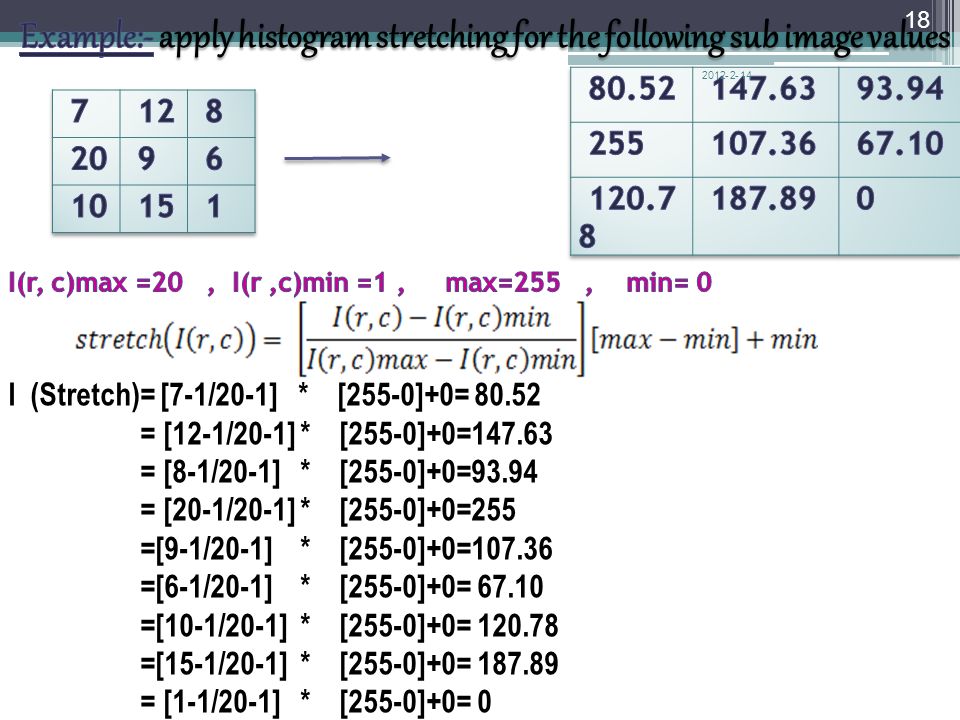
14-2-2012 16 I(r, c)max is the largest gray-level value in the image I(r, c) I(r, c)min is the smallest gray level value in the image I(r, c) Max and min correspond to the maximum and minimum gray-level values possible(for 8-bit image these are 255 and 0)
max is the largest gray-level value in the image I(r, c) I(r, c)min is the smallest gray level value in the image I(r, c) Max and min correspond to the maximum and minimum gray-level values possible(for 8-bit image these are 255 and 0)")
18
14-2-2012 17
19
14-2-2012 18
20
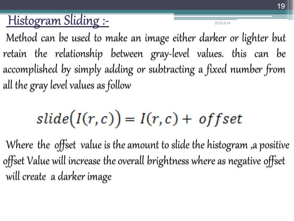
Where the offset value is the amount to slide the histogram,a positive offset Value will increase the overall brightness where as negative offset will create a darker image 14-2-2012 19

21
14-2-2012 20

22
Slide(I(r, c)) = 7+10 = 17 =12+10 = 22 = 8+10 = 18 = 20+10 = 130 =9+10 = 19 =6+10 = 16 = 10+10 = 20 = 15+10 = 25 = 1+10 = 11 14-2-2012 21
) = 7+10 = 17 =12+10 = 22 = 8+10 = 18 = = 130 =9+10 = 19 =6+10 = 16 = = 20 = = 25 = 1+10 =")
23
14-2-2012 22

24
14-2-2012 23
25
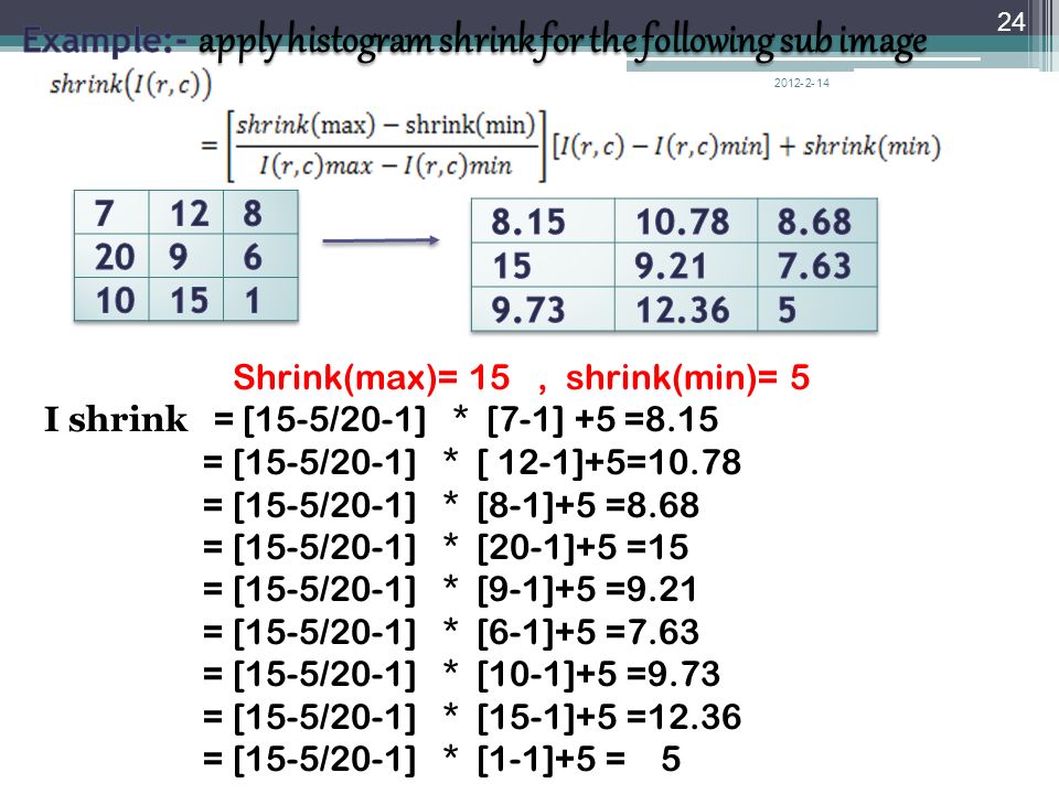
Shrink(max)= 15, shrink(min)= 5 I shrink = [15-5/20-1] * [7-1] +5 =8.15 = [15-5/20-1] * [ 12-1]+5=10.78 = [15-5/20-1] * [8-1]+5 =8.68 = [15-5/20-1] * [20-1]+5 =15 = [15-5/20-1] * [9-1]+5 =9.21 = [15-5/20-1] * [6-1]+5 =7.63 = [15-5/20-1] * [10-1]+5 =9.73 = [15-5/20-1] * [15-1]+5 =12.36 = [15-5/20-1] * [1-1]+5 = 5 14-2-2012 24
![Shrink(max)= 15, shrink(min)= 5 I shrink = [15-5/20-1] * [7-1] +5 =8.15 = [15-5/20-1] * [ 12-1]+5=10.78 = [15-5/20-1] * [8-1]+5 =8.68 = [15-5/20-1] * [20-1]+5 =15 = [15-5/20-1] * [9-1]+5 =9.21 = [15-5/20-1] * [6-1]+5 =7.63 = [15-5/20-1] * [10-1]+5 =9.73 = [15-5/20-1] * [15-1]+5 =12.36 = [15-5/20-1] * [1-1]+5 =](http://images.slideplayer.com/25/7827270/slides/slide_25.jpg "Shrink(max)= 15, shrink(min)= 5 I shrink = [15-5/20-1] * [7-1] +5 =8.15 = [15-5/20-1] * [ 12-1]+5=10.78 = [15-5/20-1] * [8-1]+5 =8.68 = [15-5/20-1] * [20-1]+5 =15 = [15-5/20-1] * [9-1]+5 =9.21 = [15-5/20-1] * [6-1]+5 =7.63 = [15-5/20-1] * [10-1]+5 =9.73 = [15-5/20-1] * [15-1]+5 =12.36 = [15-5/20-1] * [1-1]+5 =")
26
14-2-2012 25 Histogram equalization is a technique where the histogram of the resultant image is as flat as possible (with histogram stretching the overall shape of the histogram remains the same) The results in a histogram with a mountain grouped closely together to "spreading or flatting histogram makes the dark pixels appear darker and the light pixels appear lighter (the key word is "appear" the dark pixels in a photograph can not by any darker. If, however, the pixels that are only slightly lighter become much lighter, then the dark pixels will appear darker).
..")
27
14-2-2012 26
28
14-2-2012 27
29
14-2-2012 28

30
0 1 2 3 4 5 6 7 2 4 6 8 10 12 14 2 4 6 8 10 12 14 14-2-2012 29
31
14-2-2012 30

32
14-2-2012 31 0 1 2 3 4 5 6 7 1 2 3 4 5 6 7 1 2 3 4 5 6 7

33
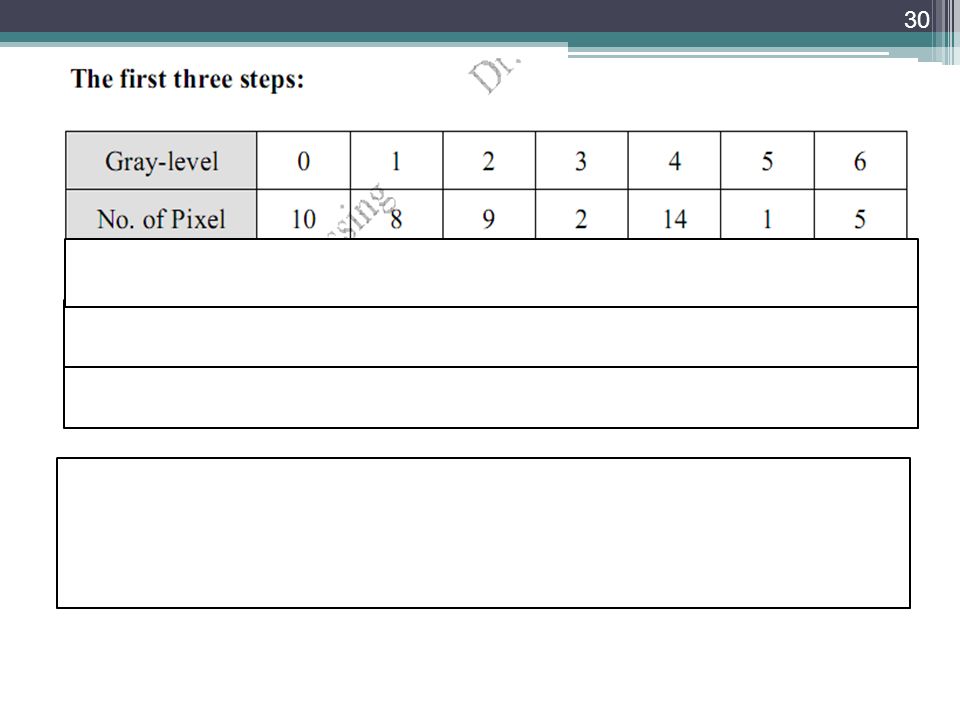
14-2-2012 32 Step 1: Great a running sum of histogram values. This means that the first values is 10, the second is 10+8=18, next is 10+8+9=27, and soon. Here we get 10,18,29,43,44,49,51. Step 2: Normalize by dividing by total number of pixels. The total number of pixels is 10+8+9+2+14+1+5+0=51. Step 3: Multiply these values by the maximum gray – level values in this case 7, and then round the result to the closet integer. After this is done we obtain 1,2,4,4,6,6,7,7. Step 4: Map the original values to the results from step3 by a one –to- one correspondence.

34
14-2-2012 33
35
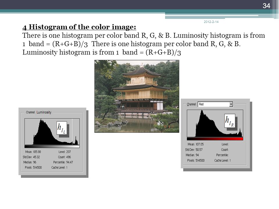
14-2-2012 34 4 Histogram of the color image: There is one histogram per color band R, G, & B. Luminosity histogram is from 1 band = (R+G+B)/3
/3.")
36
14-2-2012 35
37
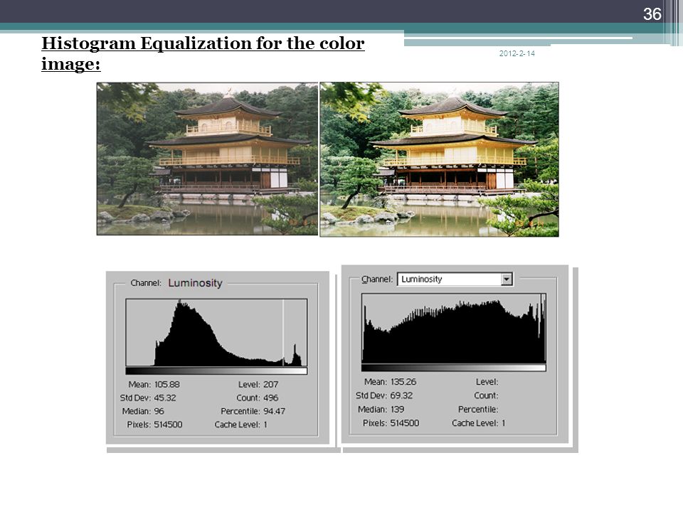
14-2-2012 36 Histogram Equalization for the color image:

Similar presentations


>")
=nk, where: rk is the kth gray level nk.>")

 Coding and Processing Lecture 5: Point Operations Wade Trappe.>")


