Download presentation
Presentation is loading. Please wait.

1
Some material taken from website of Dale Winter

2
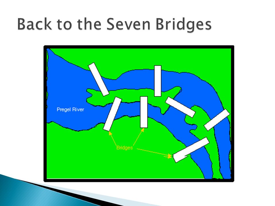
Leonhard Euler – 1736 Find a starting point so that you can walk around the city, crossing each bridge exactly once, and end up at your starting point

3
What is the smallest number of colors needed to color any planar map (drawn so that no edges cross) so that any two neighboring regions have different colors? Over the last 150 years, some big shots in the world of mathematics have been involved with this problem. Around 1850, Francis Guthrie showed how to color a map of all the counties in England using only four colors. He became interested in the general problem, and talked about it with his brother, Frederick. Frederick talked about it with his math teacher, Augustus DeMorgan, who sent the problem to William Hamilton Hamilton was evidently too interested in other and it lay dormant for about 25 years. In 1878, Arthur Cayley made the scientific community aware of the problem again, and shortly thereafter, British mathematician Sir Alfred Kempe devised a 'proof' that was unquestioned for over ten years. However, in 1890 Percy John Heawood, found a mistake in Kempe's work. The problem remained unsolved until 1976, when Kenneth Appel and Wolfgang Haken produced a proof involving an intricate computer analysis of 1936 different configurations.

4
Unlabeled graph ◦ Nodes (vertex) and links (edges), without notations on nodes Labeled graph ◦ Nodes contain a label Weighted graph ◦ Links have an associated value or “weight” label Vertex is adjacent to another if an edge connects it ◦ The vertices are called “neighbors” Path ◦ Sequence of edges, to get from one vertex to another A vertex is “reachable” if there is a path between the two nodes Length if path: number of edges on the path Connected graph ◦ A path exists from each node to every other node Complete graph ◦ Path from each vertex to every other vertex
 and links (edges), without notations on nodes Labeled graph ◦ Nodes contain a label Weighted graph ◦ Links have an associated value or weight label Vertex is adjacent to another if an edge connects it ◦ The vertices are called neighbors Path ◦ Sequence of edges, to get from one vertex to another A vertex is reachable if there is a path between the two nodes Length if path: number of edges on the path Connected graph ◦ A path exists from each node to every other node Complete graph ◦ Path from each vertex to every other vertex")
5
Degree of a vertex ◦ Number of edges connected to it In a complete graph, it number of vertices minus 1 Simple path ◦ Does not pass through a vertex more than once Cycle ◦ Path begins / ends at the same vertex Undirected ◦ Edges do not indicate a direction Directed ◦ Explicit direction in an edge between two nodes “digraph” (directed graph) ◦ Directed edges Source and destination vertices ◦ Incident edges Edges emanating from a source vertex
 ◦ Directed edges Source and destination vertices ◦ Incident edges Edges emanating from a source vertex")
6
How is a graph different from a tree? ◦ A node can have many parents in a graph ◦ Links can have values or weights assigned to them

7
Directed Acyclic Graph (DAG) ◦ Contains no cycles Lists and trees ◦ Special cases of directed graphs List ◦ Nodes are predecessors and successors Tree ◦ Nodes are parents and children
 ◦ Contains no cycles Lists and trees ◦ Special cases of directed graphs List ◦ Nodes are predecessors and successors Tree ◦ Nodes are parents and children")
8
Dense and sparse graphs ◦ Based of number of edges in the graph Limiting cases ◦ Complete directed graph with N vertices N * (N-1) ◦ Complete undirected graph with N vertices N * (N-1) / 2
 ◦ Complete undirected graph with N vertices N * (N-1) / 2")
9
Tetrahedral Octahedral Cube

10
Definition : ◦ A graph G consists of a set of vertices and a set of edges, where each edge joins an unordered pair of vertices. The set of vertices of G is denoted by V(G) and the set of edges is denoted by E(G). Definition: ◦ A loop is an edge that joins a vertex to itself. A multiple edge occurs when there is more than one edge joining a pair of vertices. Definition: ◦ A simple graph is a pair (V(G), E(G)) where V(G) is a non-empty finite set of elements, and E(G) is a finite set of unordered pairs of distinct elements of V(G).
 and the set of edges is denoted by E(G). Definition: ◦ A loop is an edge that joins a vertex to itself. A multiple edge occurs when there is more than one edge joining a pair of vertices. Definition: ◦ A simple graph is a pair (V(G), E(G)) where V(G) is a non-empty finite set of elements, and E(G) is a finite set of unordered pairs of distinct elements of V(G)..")
11
Directed graph to describe the sequence of courses (with prerequisites) Roadmap Airline routes Adventure game layout Network schematic Web page links Relationship between students and courses Flow capacities in a communications or a transportation network Neurons
 Roadmap Airline routes Adventure game layout Network schematic Web page links Relationship between students and courses Flow capacities in a communications or a transportation network Neurons")
12
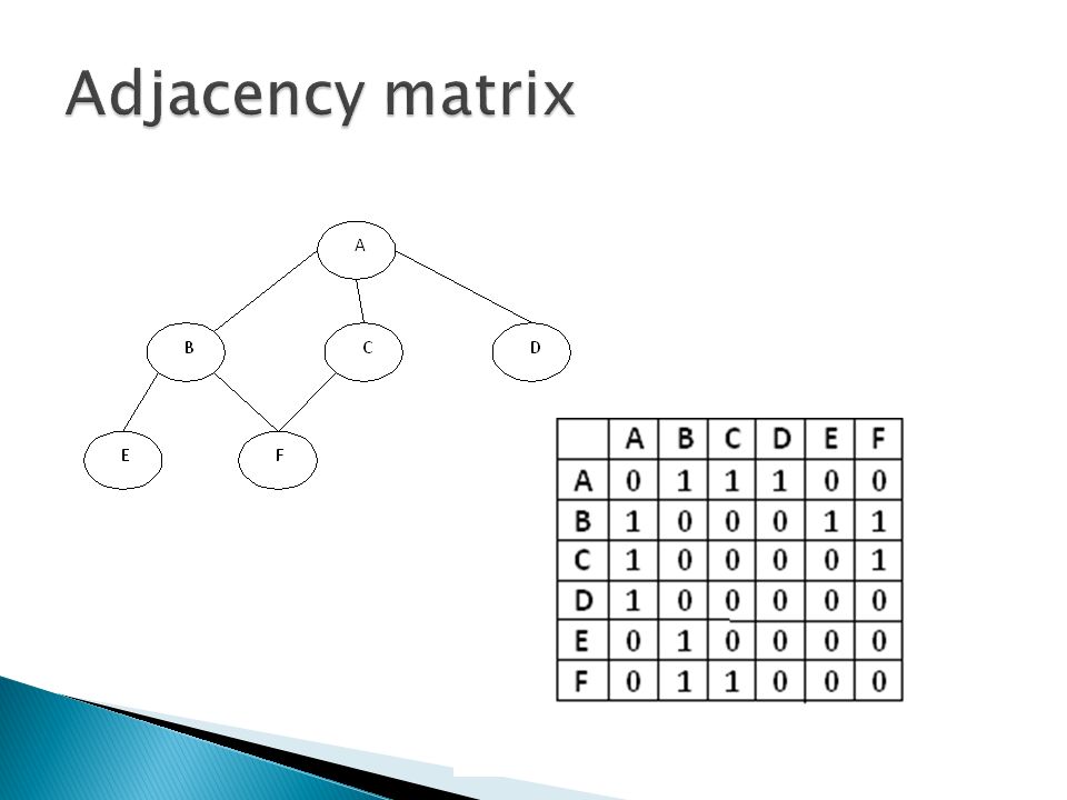
How can I represent the edges in a graph? ◦ Adjacency matrix ◦ Adjacency list

13
Adjacency matrix ◦ Using Boolean flags, we construct an n by n matrix Each node/vertex is a row/column in the matrix ◦ The flag indicates a link between the two nodes ◦ Advantages Easy to put into practice..a 2D array Adding/deleting links easy.. Just update the Boolean flags ◦ Disadvantages Memory usage as the node count increases Information redundancy

15
Directed graph 4 bidirectional links Adjacency matrix Destination Nodes Source Nodes ABCD A0100 B1011 C0101 D0110 A C B D

16
Directed graph 4 directed links Adjacency matrix 4 links Weight can occupy cell Destination Nodes Source Nodes ABCD A0000 B1001 C0100 D0010 A C B D

17
Array of Linked List nodes ◦ List whose elements are a linked list

18
Graph information stored in a matrix or grid ◦ Grid “G” ◦ We note if a vertex is “incident” to a particular edge Side 'a'Side 'b'Side 'c'Side 'd' Vertex 1 1000 Vertex 2 1101 Vertex 3 0110 Vertex 4 0011

19
Directed graph 4 directed links Weighting can also be assigned, next to the destination node A C B D

20
The number of edges incident with a vertex

21
Determine if edge exists between two vertices Find all adjacent vertices for a given vertex Consider the computational advantages in using one over the other

22
Two algorithms to traverse and search for a node Determine if a node is reachable from a given node BFS ◦ Breadth First Search DFS ◦ Depth First Search

23
See how far you can go ◦ Use a STACK Result is A B E F C D 1.Push root node 2.Loop until the stack is empty 3.Peek the node in the stack 4.If node has unvisited child nodes, mark as traversed and push it on stack 5.If node does not have unvisited child nodes, pop the node from the stack

24
public void dfs() {//DFS uses Stack data structure Stack s=new Stack(); s.push(this.rootNode); rootNode.visited=true; printNode(rootNode); while(!s.isEmpty()) {Node n=(Node)s.peek(); Node child=getUnvisitedChildNode(n); if (child!=null) { child.visited=true; printNode(child); s.push(child); } else { s.pop(); } //Clear visited property of nodes clearNodes();}
 {//DFS uses Stack data structure Stack s=new Stack(); s.push(this.rootNode); rootNode.visited=true; printNode(rootNode); while(!s.isEmpty()) {Node n=(Node)s.peek(); Node child=getUnvisitedChildNode(n); if (child!=null) { child.visited=true; printNode(child); s.push(child); } else { s.pop(); } //Clear visited property of nodes clearNodes();}")
25
Stay close to root ◦ Visit “level” by “level” ◦ Use a QUEUE Result is A B C D E F 1.Push root node into the queue 2.Loop until the queue is empty 3.Remove the node from the queue 4.If removed node has unvisited child nodes, mark as traversed and insert unvisited children into queue

26
public void bfs() {//BFS uses Queue data structure Queue q=new LinkedList(); q.add(this.rootNode); printNode(this.rootNode); rootNode.visited=true; while(!q.isEmpty()) { Node n=(Node)q.remove(); Node child=null; while ((child=getUnvisitedChildNode(n))!=null) { child.visited=true; printNode(child); q.add(child); } //Clear visited property of nodes clearNodes();}
 {//BFS uses Queue data structure Queue q=new LinkedList(); q.add(this.rootNode); printNode(this.rootNode); rootNode.visited=true; while(!q.isEmpty()) { Node n=(Node)q.remove(); Node child=null; while ((child=getUnvisitedChildNode(n))!=null) { child.visited=true; printNode(child); q.add(child); } //Clear visited property of nodes clearNodes();}")
27
Follow a sequence of links Operations ◦ Insert/delete items in the graph ◦ Find the shortest path to a given item in a graph ◦ Find all items to which a given item is connected in a graph ◦ Traverse all of the items in a graph

28
Starting with an arbitrary vertex TraverseFromVertex(graph, startVertex) Mark all vertices as unvisited Insert startVertex into empty collection While (collection not empty) Remove a vertex from the collection If vertex hasn’t been visited Mark it as visited Process the vertex Insert all adjacent unvisited vertices into the collection
 Mark all vertices as unvisited Insert startVertex into empty collection While (collection not empty) Remove a vertex from the collection If vertex hasn’t been visited Mark it as visited Process the vertex Insert all adjacent unvisited vertices into the collection")
29
All vertices reachable from startVertex are processed exactly once Determining adjacent vertices is straightforward ◦ Matrix used: Iterate across the vertex’s row ◦ List used: Traverse the vertex’s linked list

30
Depth-first ◦ Uses a stack as a collection Goes deeply before backtracking to another path ◦ Can be implemented recursively Breadth-first ◦ Queue is the collection Visit every adjacent vertex before proceeding deeper Similar to a level order traversal of a tree

31
Graph can be partitioned into disjoint components ◦ Each component stored in a set Sets are stored in a list

32
Spanning Tree ◦ Fewest number of edges possible While keeping connection between all vertices in the component N – 1 edges in the tree for “N” vertices ◦ Traversing all the vertices of an undirected graph (not just a single component) Generates a spanning forest
 Generates a spanning forest")
33
Weighted edges ◦ Sum all edges Minimize the sum Minimum spanning forest ◦ Applies to the entire graph Algorithms ◦ 1957: Prim’s algorithm ◦ 1956: Kurskal’s algorithm Prim’s algorithm (We are assuming a connected graph) Mark all vertices and edges as unvisited Mark vertex “v” as visited For all vertices Find the least weight edge from a visited vertex to an unvisited vertex Mark the edge and vertex as unvisited At the end, the edges are the tree’s branches in the minimum spanning tree
 Mark all vertices and edges as unvisited Mark vertex v as visited For all vertices Find the least weight edge from a visited vertex to an unvisited vertex Mark the edge and vertex as unvisited At the end, the edges are the tree’s branches in the minimum spanning tree")
34
DAG ◦ Topological order assigns a rank to each vertex Edges go from lower to higher ranked vertices Sort based on graph traversal Either depth or breadth based Vertices are returned in a stack in ascending order

35
Single source shortest path problem ◦ Shortest path from a single vertex to all other vertices Dijkstra’s algorithm Assumes all weights are positive All-pairs shortest path problem ◦ Set of all shortest paths I a graph

36
Computes distances of the shortest paths fro a source vertex to all other vertices in the graph Output is a 2D grid (called “results”) ◦ N rows First column in each row is a vertex Second column is the distance from source to this vertex Third column holds the immediate parent vertex on this path ◦ Temporary list, called “included” produced Contains N Booleans Tracks if a vertex has been included in the set of vertices for which we’ve already determined the shortest path
 ◦ N rows First column in each row is a vertex Second column is the distance from source to this vertex Third column holds the immediate parent vertex on this path ◦ Temporary list, called included produced Contains N Booleans Tracks if a vertex has been included in the set of vertices for which we’ve already determined the shortest path")
38
The bridges are “pairs” of vertices joined by edges

39
Complete the graph ◦ Draw in the joining streets

40
“Bridge” edges are in blue Do we have a sequence of edges so that: ◦ Consecutive edges e j … and e j+1 are incident to a common vertex AND Each of the blue edges belongs to the sequence AND Each of the blue edges occurs exactly one in the sequence Referred to as a “walk”

42
Walk ◦ Finite sequence of edges, e 1,..., e m ◦ edge, e j, incident to vertices v j - 1 and v j such that any two consecutive edges e j and e j + 1 are incident to a common vertex v j ◦ vertex v 0 is called the initial vertex and the vertex v m is called the final vertex ◦ number of edges in the walk is called the length of the walk

43
In a walk, no requirement that edges in walk are different from each other ◦ possible to have a walk that consists of same edge repeated over and over Like walking up and down the same street over and over Assumption that all edges in the walk are distinct ◦ Definition of a PATH Closed walk ◦ Walk from a vertex to itself Simple path ◦ All vertices are distinct Circuit ◦ Simple path which is closed

Similar presentations

 Lecture 3 MAS 714 part 2 Hartmut Klauck.>")


 of the depth-first search. Topological.>")


>")


 GRAPH. Introduction of Graph A graph G consists of two things: 1.A set V of elements called nodes(or points or.>")


