1. Orthogonal Linear Contrasts This is a technique for partitioning ANOVA sum of squares into individual degrees of freedom

2. Definition Let x 1, x 2,..., x p denote p numerical quantities computed from the data. These could be statistics or the raw observations. A linear combination of x 1, x 2,..., x p is defined to be a quantity,L,computed in the following manner: L = c 1 x 1 + c 2 x 2 +... + c p x p where the coefficients c 1, c 2,..., c p are predetermined numerical values:

3. Definition If the coefficients c 1, c 2,..., c p satisfy: c 1 + c 2 +... + c p = 0, Then the linear combination L = c 1 x 1 + c 2 x 2 +... + c p x p is called a linear contrast.

4. Examples 1. 2. 3.L = x 1 - 4 x 2 + 6x 3 - 4 x 4 + x 5 = (1)x 1 + (-4)x 2 + (6)x 3 + (-4)x 4 + (1)x 5 A linear combination A linear contrast

5. Definition Let A = a 1 x 1 + a 2 x 2 +... + a p x p and B= b 1 x 1 + b 2 x 2 +... + b p x p be two linear contrasts of the quantities x 1, x 2,..., x p. Then A and B are c called Orthogonal Linear Contrasts if in addition to: a 1 + a 2 +... + a p = 0 and b 1 + b 2 +... + b p = 0, it is also true that: a 1 b 1 + a 2 b 2 +... + a p b p = 0..

6. Example Let Note:

7. Definition Let A = a 1 x 1 + a 2 x 2 +... + a p x p, B= b 1 x 1 + b 2 x 2 +... + b p x p,..., and L= l 1 x 1 + l 2 x 2 +... + l p x p be a set linear contrasts of the quantities x 1, x 2,..., x p. Then the set is called a set of Mutually Orthogonal Linear Contrasts if each linear contrast in the set is orthogonal to any other linear contrast..

8. Theorem: The maximum number of linear contrasts in a set of Mutually Orthogonal Linear Contrasts of the quantities x 1, x 2,..., x p is p - 1. p - 1 is called the degrees of freedom (d.f.) for comparing quantities x 1, x 2,..., x p.

9. Comments 1.Linear contrasts are making comparisons amongst the p values x 1, x 2,..., x p 2.Orthogonal Linear Contrasts are making independent comparisons amongst the p values x 1, x 2,..., x p. 3.The number of independent comparisons amongst the p values x 1, x 2,..., x p is p – 1.

10. Definition denotes a linear contrast of the p means If each mean,, is calculated from n observations then: The Sum of Squares for testing the Linear Contrast L, is defined to be:

11. the degrees of freedom (df) for testing the Linear Contrast L, is defined to be the F-ratio for testing the Linear Contrast L, is defined to be:

12. Theorem: Let L 1, L 2,..., L p-1 denote p-1 mutually orthogonal Linear contrasts for comparing the p means. Then the Sum of Squares for comparing the p means based on p – 1 degrees of freedom, SS Between, satisfies:

13. Comment Defining a set of Orthogonal Linear Contrasts for comparing the p means allows the researcher to "break apart" the Sum of Squares for comparing the p means, SS Between, and make individual tests of each the Linear Contrast.

14. The Diet-Weight Gain example The sum of Squares for comparing the 6 means is given in the Anova Table:

15. Five mutually orthogonal contrasts are given below (together with a description of the purpose of these contrasts) : (A comparison of the High protein diets with Low protein diets) (A comparison of the Beef source of protein with the Pork source of protein)

16. (A comparison of the Meat (Beef - Pork) source of protein with the Cereal source of protein) (A comparison representing interaction between Level of protein and Source of protein for the Meat source of Protein) (A comparison representing interaction between Level of protein with the Cereal source of Protein)

17. The Anova Table for Testing these contrasts is given below: The Mutually Orthogonal contrasts that are eventually selected should be determine prior to observing the data and should be determined by the objectives of the experiment

18. Another Five mutually orthogonal contrasts are given below (together with a description of the purpose of these contrasts) : (A comparison of the Beef source of protein with the Pork source of protein) (A comparison of the Meat (Beef - Pork) source of protein with the Cereal source of protein)

19. (A comparison of the high and low protein diets for the Beef source of protein) (A comparison of the high and low protein diets for the Cereal source of protein) (A comparison of the high and low protein diets for the Pork source of protein)

20. The Anova Table for Testing these contrasts is given below:

21. Orthogonal Linear Contrasts Polynomial Regression

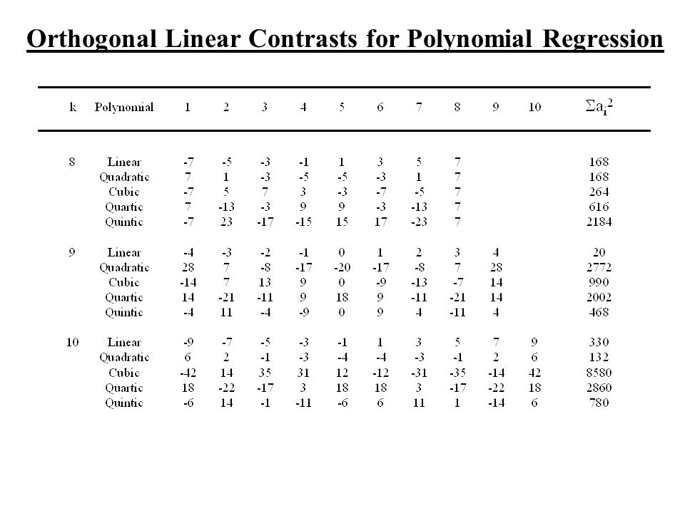
22. Orthogonal Linear Contrasts for Polynomial Regression

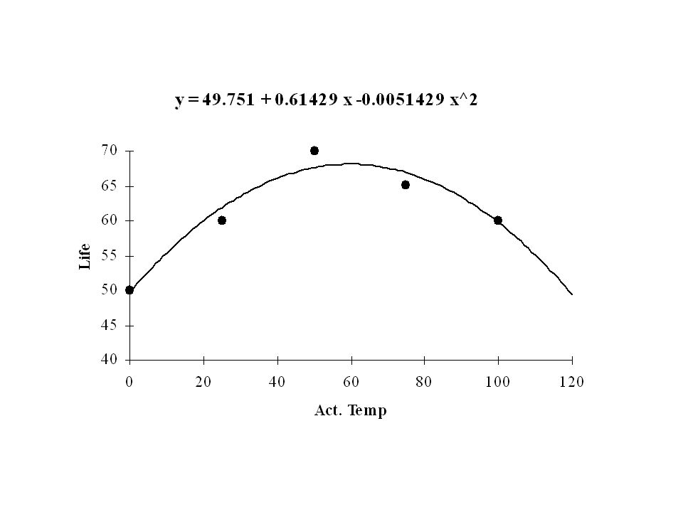
24. Example In this example we are measuring the “Life” of an electronic component and how it depends on the temperature on activation

25. The Anova Table SourceSSdfMSF Treat6604165.023.57 Linear187.501187.5026.79 Quadratic433.931433.9361.99 Cubic0.0010.000.00 Quartic38.57138.575.51 Error70107.00 Total73014 L = 25.00Q 2 = -45.00C = 0.00Q 4 = 30.00

26. The Anova Tables for Determining degree of polynomial Testing for effect of the factor

27. Testing for departure from Linear

28. Testing for departure from Quadratic

30. Multiple Testing Tukey’s Multiple comparison procedure Scheffe’s multiple comparison procedure

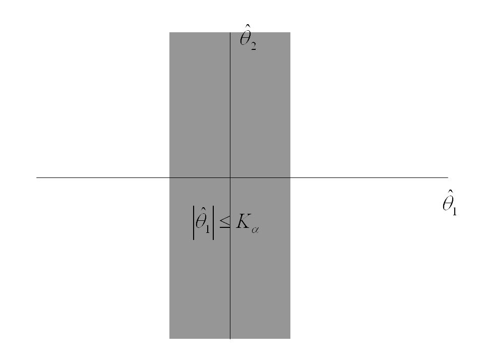
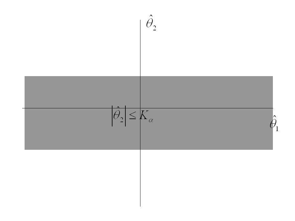
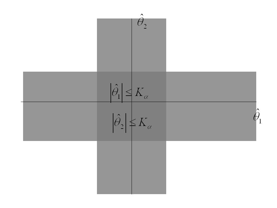
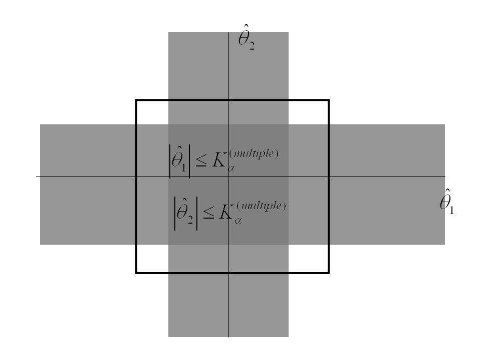
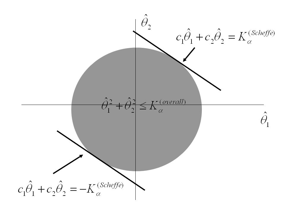
31. Multiple Testing – a Simple Example Suppose we are interested in testing to see if two parameters (  1 and  2 ) are equal to zero. There are two approaches 1.We could test each parameter separately a) H 0 :  1 = 0 against H A :  1 ≠ 0, then b)H 0 :  2 = 0 against H A :  2 ≠ 0 2.We could develop an overall test H 0 :  1 = 0,  2 = 0 against H A :  1 ≠ 0 or  2 ≠ 0

32. 1.To test each parameter separately a) then b) We might use the following test: then is chosen so that the probability of a Type I errorof each test is .

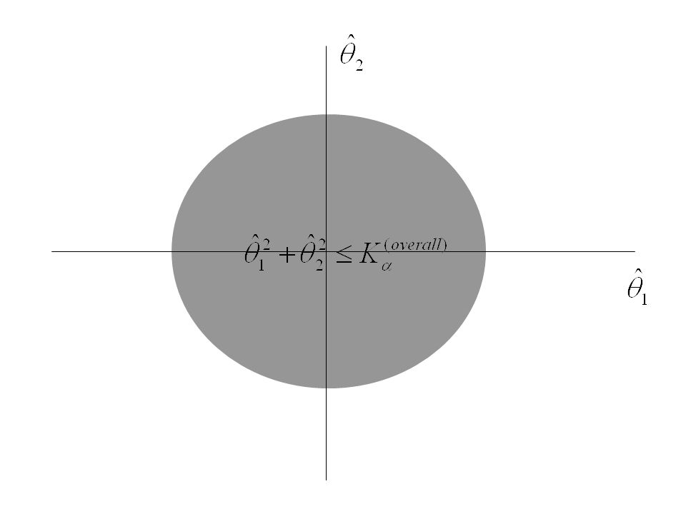
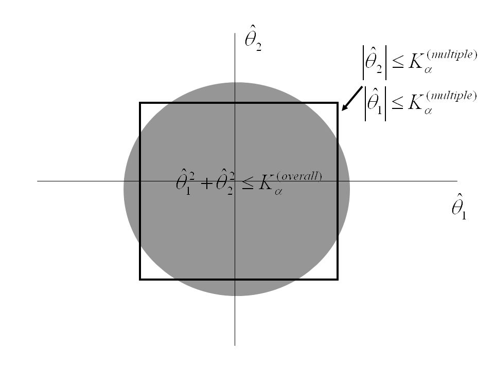
33. 2.To perform an overall test H 0 :  1 = 0,  2 = 0 against H A :  1 ≠ 0 or  2 ≠ 0 we might use the test is chosen so that the probability of a Type I error is .

41. Post-hoc Tests Multiple Comparison Tests

42. Post-hoc Tests Multiple Comparison Tests

43. Suppose we have p means An F-test has revealed that there are significant differences amongst the p means We want to perform an analysis to determine precisely where the differences exist.

44. Tukey’s Multiple Comparison Test

45. Let Tukey's Critical Differences Two means are declared significant if they differ by more than this amount. denote the standard error of each = the tabled value for Tukey’s studentized range p = no. of means, = df for Error

46. Scheffe’s Multiple Comparison Test

47. Scheffe's Critical Differences (for Linear contrasts) A linear contrast is declared significant if it exceeds this amount. = the tabled value for F distribution (p -1 = df for comparing p means, = df for Error)

48. Scheffe's Critical Differences (for comparing two means) Two means are declared significant if they differ by more than this amount.

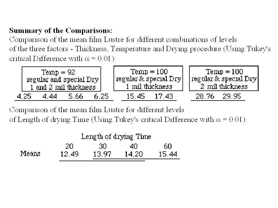
51. Underlined groups have no significant differences

52. There are many multiple (post hoc) comparison procedures 1.Tukey’s 2.Scheffe’, 3.Duncan’s Multiple Range 4.Neumann-Keuls etc Considerable controversy: “I have not included the multiple comparison methods of D.B. Duncan because I have been unable to understand their justification” H. Scheffe, Analysis of Variance