Download presentation
Presentation is loading. Please wait.

1
Lecture 11: Networks II: conductance-based synapses, visual cortical hypercolumn model References: Hertz, Lerchner, Ahmadi, q-bio.NC/0402023 [Erice lectures] Lerchner, Ahmadi, Hertz, q-bio.NC/0402026 (Neurocomputing, 2004) [conductance-based synapses] Lerchner, Sterner, Hertz, Ahmadi, q-bio.NC/0403037 [orientation hypercolumn model]
![Lecture 11: Networks II: conductance-based synapses, visual cortical hypercolumn model References: Hertz, Lerchner, Ahmadi, q-bio.NC/ [Erice lectures] Lerchner, Ahmadi, Hertz, q-bio.NC/ (Neurocomputing, 2004) [conductance-based synapses] Lerchner, Sterner, Hertz, Ahmadi, q-bio.NC/ [orientation hypercolumn model]](http://images.slideplayer.com/25/7797836/slides/slide_1.jpg "Lecture 11: Networks II: conductance-based synapses, visual cortical hypercolumn model References: Hertz, Lerchner, Ahmadi, q-bio.NC/ [Erice lectures] Lerchner, Ahmadi, Hertz, q-bio.NC/ (Neurocomputing, 2004) [conductance-based synapses] Lerchner, Sterner, Hertz, Ahmadi, q-bio.NC/ [orientation hypercolumn model]")
2
Conductance-based synapses In previous model:

3
Conductance-based synapses In previous model: But a synapse is a channel with a (neurotransmitter-gated) conductance:
 conductance:")
4
Conductance-based synapses In previous model: But a synapse is a channel with a (neurotransmitter-gated) conductance:
 conductance:")
5
Conductance-based synapses In previous model: But a synapse is a channel with a (neurotransmitter-gated) conductance: whereis the synaptically-filtered presynaptic spike train
 conductance: whereis the synaptically-filtered presynaptic spike train")
6
Conductance-based synapses In previous model: But a synapse is a channel with a (neurotransmitter-gated) conductance: whereis the synaptically-filtered presynaptic spike train kernel:
 conductance: whereis the synaptically-filtered presynaptic spike train kernel:")
7
Conductance-based synapses In previous model: But a synapse is a channel with a (neurotransmitter-gated) conductance: whereis the synaptically-filtered presynaptic spike train kernel:
 conductance: whereis the synaptically-filtered presynaptic spike train kernel:")
8
Conductance-based synapses In previous model: But a synapse is a channel with a (neurotransmitter-gated) conductance: whereis the synaptically-filtered presynaptic spike train kernel:
 conductance: whereis the synaptically-filtered presynaptic spike train kernel:")
9
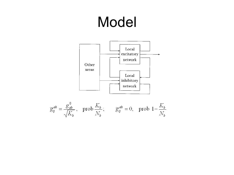
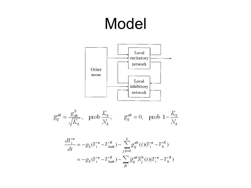
Model

12
Mean field theory Effective single-neuron problem with synaptic input current

13
Mean field theory Effective single-neuron problem with synaptic input current

14
Mean field theory Effective single-neuron problem with synaptic input current with

15
Mean field theory Effective single-neuron problem with synaptic input current with where = correlation function of synaptically-filtered presynaptic spike trains

16
Balance condition Total mean current = 0 :

17
Balance condition Total mean current = 0 :

18
Balance condition Total mean current = 0 : Mean membrane potential just below

19
Balance condition define Total mean current = 0 : Mean membrane potential just below

20
Balance condition define Total mean current = 0 : Mean membrane potential just below

21
Balance condition define Solve for r b as in current-based case: Total mean current = 0 : Mean membrane potential just below

22
Balance condition define Solve for r b as in current-based case: Total mean current = 0 : Mean membrane potential just below

23
Balance condition define Solve for r b as in current-based case: Total mean current = 0 : Mean membrane potential just below

24
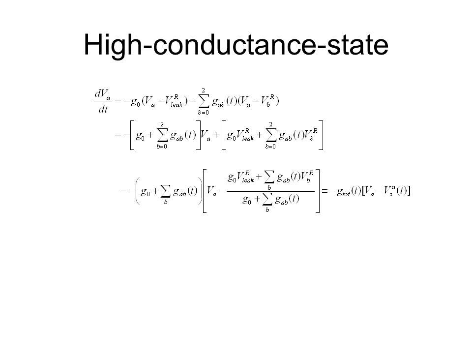
High-conductance-state

26
V a “chases” V s a (t) at rate g tot (t)
 at rate g tot (t)")
27
High-conductance-state V a “chases” V s a (t) at rate g tot (t)
 at rate g tot (t)")
28
High-conductance-state V a “chases” V s a (t) at rate g tot (t)
 at rate g tot (t)")
29
High-conductance-state V a “chases” V s a (t) at rate g tot (t) Effective membrane time constant ~ 1 ms
 at rate g tot (t) Effective membrane time constant ~ 1 ms")
30
Membrane potential and spiking dynamics for large g tot

31
Fluctuations Measure membrane potential from :

32
Fluctuations Measure membrane potential from :

33
Fluctuations Measure membrane potential from : Conductances: mean + fluctuations:

34
Fluctuations Measure membrane potential from : Conductances: mean + fluctuations:

35
Fluctuations Measure membrane potential from : Conductances: mean + fluctuations:

36
Fluctuations Measure membrane potential from : Use balance equation in Conductances: mean + fluctuations:

37
Fluctuations Measure membrane potential from : Use balance equation in Conductances: mean + fluctuations: =>

38
Fluctuations Measure membrane potential from : Use balance equation in Conductances: mean + fluctuations: => or

39
Fluctuations Measure membrane potential from : Use balance equation in Conductances: mean + fluctuations: => or with

40
Fluctuations Measure membrane potential from : Use balance equation in Conductances: mean + fluctuations: => or with

41
Effective current-based model High connectivity:

42
Effective current-based model High connectivity:

43
Effective current-based model High connectivity:

44
Effective current-based model High connectivity:

45
Effective current-based model High connectivity:

46
Effective current-based model High connectivity: Like current-based model with

47
Effective current-based model High connectivity: Like current-based model with (but effective membrane time constant depends on presynaptic rates)
")
48
Firing irregularity depends on reset level and s

49
Modeling primary visual cortex

50
Background: 1.Neurons in primary visual cortex (area V1) respond strongly to oriented stimuli (bars, gratings)
 respond strongly to oriented stimuli (bars, gratings)")
51
Modeling primary visual cortex Background: 1.Neurons in primary visual cortex (area V1) respond strongly to oriented stimuli (bars, gratings)
 respond strongly to oriented stimuli (bars, gratings)")
52
Modeling primary visual cortex Background: 1.Neurons in primary visual cortex (area V1) respond strongly to oriented stimuli (bars, gratings) Note: contrast- invariant tuning width
 respond strongly to oriented stimuli (bars, gratings) Note: contrast- invariant tuning width")
53
Spatial organization of area V1 2. In V1, nearby neurons have similar orientation tuning

54
Spatial organization of area V1 2. In V1, nearby neurons have similar orientation tuning

55
Orientation column ~ 10 4 neurons that respond most strongly to a particular orientation

56
Orientation column ~ 10 4 neurons that respond most strongly to a particular orientation Tuning of input from LGN (Hubel-Wiesel):
:")
57
Hubel-Wiesel feedforward connectivity cannot by itself explain contrast-invariant tuning Simplest model: cortical neurons sums H-W inputs, firing rate is threshold-linear function of sum

58
Hubel-Wiesel feedforward connectivity cannot by itself explain contrast-invariant tuning Simplest model: cortical neurons sums H-W inputs, firing rate is threshold-linear function of sum

59
Modeling a “hypercolumn” in V1 Coupled collection of networks, each representing an “orientation column”

60
Modeling a “hypercolumn” in V1 Coupled collection of networks, each representing an “orientation column”

61
Modeling a “hypercolumn” in V1 Coupled collection of networks, each representing an “orientation column”

62
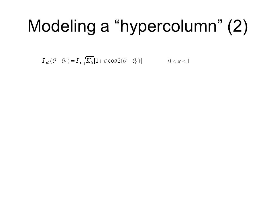
Modeling a “hypercolumn” (2)
")
64
0 is stimulus orientation

65
Modeling a “hypercolumn” (2) 0 is stimulus orientation (simplest model periodic in with period )
 0 is stimulus orientation (simplest model periodic in with period )")
66
Modeling a “hypercolumn” (2) 0 is stimulus orientation (simplest model periodic in with period )
 0 is stimulus orientation (simplest model periodic in with period )")
67
Modeling a “hypercolumn” (2) 0 is stimulus orientation (simplest model periodic in with period )
 0 is stimulus orientation (simplest model periodic in with period )")
68
Modeling a “hypercolumn” (2) 0 is stimulus orientation Connection probability falls off with increasing ’, reflecting probable greater distance. (simplest model periodic in with period )
.")
69
Mean field theory Effective intracortical input current

70
Mean field theory Effective intracortical input current mean

71
Mean field theory Effective intracortical input current mean fluctuations:

72
Mean field theory Effective intracortical input current mean fluctuations: with

73
Mean field theory Effective intracortical input current mean fluctuations: with Solve self-consistently for order parameters

74
Balance condition Total mean current vanishes at all :

75
Balance condition Total mean current vanishes at all :

76
Balance condition Total mean current vanishes at all : Ignore leak, make continuum approximation:

77
Balance condition Total mean current vanishes at all : Ignore leak, make continuum approximation:

78
Balance condition Total mean current vanishes at all : Ignore leak, make continuum approximation: Integral equations for r a ( )
")
79
Balance condition Total mean current vanishes at all : Ignore leak, make continuum approximation: Integral equations for r a ( ) Can take 0 = 0
 Can take 0 = 0")
80
Broad tuning

81
Make ansatz

82
Broad tuning Make ansatz use

83
Broad tuning Make ansatz use

84
Broad tuning Make ansatz use => with

85
Broad tuning Make ansatz use => with Solve for Fourier components:

86
Broad tuning Make ansatz use => with Solve for Fourier components:

87
Broad tuning Make ansatz use => with Solve for Fourier components: Valid for (otherwise r a ( ) < 0 at large )
 < 0 at large )")
88
narrow tuning useonly for

89
narrow tuning useonly for i.e.,

90
narrow tuning useonly for i.e., same c for both populations – consequence of

91
narrow tuning useonly for i.e., same c for both populations – consequence of same for both populations in

92
narrow tuning useonly for i.e., same c for both populations – consequence of same for both populations in and same for all interactions in

93
narrow tuning useonly for i.e., same c for both populations – consequence of same for both populations in and same for all interactions in Balance condition:

94
narrow tuning useonly for i.e., same c for both populations – consequence of same for both populations in and same for all interactions in Balance condition: =>

95
Narrow tuning (2) Now do the integrals:
 Now do the integrals:")
96
Narrow tuning (2) Now do the integrals:
 Now do the integrals:")
97
Narrow tuning (2) Now do the integrals: where
 Now do the integrals: where")
98
Narrow tuning (2) Now do the integrals: where f0:f2:f0:f2: ______ ----------
 Now do the integrals: where f0:f2:f0:f2: ______")
99
Narrow tuning (3)
")
100
Divide one by the other:

101
Narrow tuning (3) Divide one by the other: determines c
 Divide one by the other: determines c")
102
Narrow tuning (3) Divide one by the other: determines c c is independent of I a0 : contrast-invariant tuning width (as in experiments)
 Divide one by the other: determines c c is independent of I a0 : contrast-invariant tuning width (as in experiments)")
103
Narrow tuning (3) Divide one by the other: determines c c is independent of I a0 : contrast-invariant tuning width (as in experiments) Then can solve for rate components:
 Divide one by the other: determines c c is independent of I a0 : contrast-invariant tuning width (as in experiments) Then can solve for rate components:")
104
Narrow tuning (3) Divide one by the other: determines c c is independent of I a0 : contrast-invariant tuning width (as in experiments) Then can solve for rate components:
 Divide one by the other: determines c c is independent of I a0 : contrast-invariant tuning width (as in experiments) Then can solve for rate components:")
105
Noise tuning Input noise correlations:

106
Noise tuning Input noise correlations:

107
Noise tuning Input noise correlations:

108
Noise tuning Input noise correlations: =>

109
Noise tuning Input noise correlations: => Same integrals as in rate computation =>

110
Noise tuning Input noise correlations: => Same integrals as in rate computation =>

111
Noise tuning Input noise correlations: => Same integrals as in rate computation => using

112
Noise tuning Input noise correlations: => Same integrals as in rate computation => using=>

113
Noise tuning Input noise correlations: => Same integrals as in rate computation => using=>Same tuning as input!

114
Some numerical results (1)
")
115
Numerical results (2): Fano factor tuning
: Fano factor tuning")
116
Numerical results (3): noise tuning vs firing tuning
: noise tuning vs firing tuning")
Similar presentations


 N Brunel, Network 11, 261-280 (2000) N Brunel, Cerebral.>")
![III-28 [122] Spike Pattern Distributions in Model Cortical Networks Joanna Tyrcha, Stockholm University, Stockholm; John Hertz, Nordita, Stockholm/Copenhagen.](/15/4642362/big_thumb.jpg "III-28 [122] Spike Pattern Distributions in Model Cortical Networks Joanna Tyrcha, Stockholm University, Stockholm; John Hertz, Nordita, Stockholm/Copenhagen.>")


 Jaime de la Rocha (NYU, Rutgers) Peter Bartho (Rutgers) Liad Hollender (Rutgers) Néstor Parga (UA Madrid)>")


>")


 Lecture 12 Course: Neural Networks and Biological Modeling Wulfram.>")