Download presentation
Presentation is loading. Please wait.

1
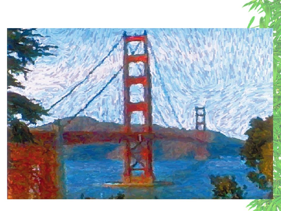
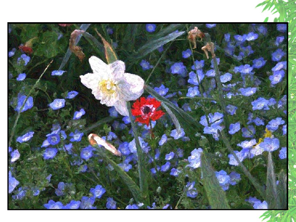
Processing Images and Video for an Impressionist Effect Author: Peter Litwinowicz Presented by Jing Yi Jin

2
Objective Generate the a hand-drawn animation from video clip automatically Impressionist style Intervention from the user in the first frame Exploit the temporal coherence Input Output Video clip Hand-drawn impressionist style animation

3
Inspiration “Catch the fleeting impression of sunlight on objects. And it was this out-of-doors world he wanted to capture in paint – as it actually was at the moment of seeing it, not worked up in the studio from sketches.” --- Kringston

4
Advantages Presents a process that uses optical flow fields to generate the animation The first to produce a temporally coherent painterly animation … Describes a new technique to orient strokes from frame- to-frame Uses algorithms to manage the stroke density

5
Structure of the presentation Previous works Previous works Current algorithm –Stroke rendering and clippingStroke rendering and clipping –Stroke orientationStroke orientation –AnimationAnimation Conclusion Conclusion

6
Previous works Hieberli, 90 –Computer-assisted transformation of picturesComputer-assisted transformation of pictures Extensive human interaction Specify the number, position of stroke Orientation, size, color of stroke controlled in an interactive or non-interactive way Static images only Difficult in extend it to deal with a sequence of images Inspiration: modify this approach to produce temporal coherent animation

7
Previous works (2) Salisbury, 94 and 96 –Pen-ink pattern –Picture controlled either in an interactive or non- interactive way Static image only Temporally coherence not straightforward Perceived edge preserved
 Salisbury, 94 and 96 –Pen-ink pattern –Picture controlled either in an interactive or non- interactive way Static image only Temporally coherence not straightforward Perceived edge preserved")
8
Previous works (3) Hsu, 94 –“skeletal strokes” –Skeletal strokes are used to produce 2-1/2 D animation All animation is key-framed by the user
 Hsu, 94 – skeletal strokes –Skeletal strokes are used to produce 2-1/2 D animation All animation is key-framed by the user")
9
Previous works (4) Meier, 96 –Transforming 3D geometry into animations Temporal coherence is both interesting and important Inspiration: Video sequence as the input
 Meier, 96 –Transforming 3D geometry into animations Temporal coherence is both interesting and important Inspiration: Video sequence as the input")
10
Rendering strokes Generate strokes that cover the output image

11
Rendering strokes Stroke – an antialiased line with –Center at (cx, cy) –Length length –Thickness radius –Orientation theta
 –Length length –Thickness radius –Orientation theta")
12
Rendering strokes –User-defined initial spacing distance –Bilinearly interpolated color of the original image at (cx, cy) –Color range [0,255] –Randomized stroke order (cx,cy)
![Rendering strokes –User-defined initial spacing distance –Bilinearly interpolated color of the original image at (cx, cy) –Color range [0,255] –Randomized stroke order (cx,cy)](http://images.slideplayer.com/25/7791846/slides/slide_12.jpg "Rendering strokes –User-defined initial spacing distance –Bilinearly interpolated color of the original image at (cx, cy) –Color range [0,255] –Randomized stroke order (cx,cy)")
13
Rendering strokes Random perturbations –Assign length to length – radius to radius –Perturb color by r, g, b, each in the range [-15, 15] –Scale the perturbed color by intensity, in the range [.85, 1.15] –Clamp the resulted color to [0,255] –Perturb theta by theta in the range [-15°, 15°] –All the information is stored in a data structure
![Rendering strokes Random perturbations –Assign length to length – radius to radius –Perturb color by r, g, b, each in the range [-15, 15] –Scale the perturbed color by intensity, in the range [.85, 1.15] –Clamp the resulted color to [0,255] –Perturb theta by theta in the range [-15°, 15°] –All the information is stored in a data structure](http://images.slideplayer.com/25/7791846/slides/slide_13.jpg "Rendering strokes Random perturbations –Assign length to length – radius to radius –Perturb color by r, g, b, each in the range [-15, 15] –Scale the perturbed color by intensity, in the range [.85, 1.15] –Clamp the resulted color to [0,255] –Perturb theta by theta in the range [-15°, 15°] –All the information is stored in a data structure")
14
Clipping and rendering To preserve detail and silhouettes Inspired by Salisbury 94 – strokes are clipped to the edge provided by user No user interaction Image processing techniques to locate edges

15
Clipping and rendering

16
Algorithm: 1.Derive an intensity image: (30*r+59*g+11*b)/100 2.Blur the intensity image with a Gaussian kernel – Reduce noise –Larger kernel lost of detail –Smaller kernel retain noise – Kernel width specified by the user Kernel with the radius of 11
/100 2.Blur the intensity image with a Gaussian kernel – Reduce noise –Larger kernel lost of detail –Smaller kernel retain noise – Kernel width specified by the user Kernel with the radius of 11")
17
Clipping and rendering 3.Filter the resulting image by Sobel filter: Sobel(x,y) = Magnitude (Gx, Gy) where (Gx,Gy) = [ dI(x,y)/dx, dI(x,y)/dy ]
![Clipping and rendering 3.Filter the resulting image by Sobel filter: Sobel(x,y) = Magnitude (Gx, Gy) where (Gx,Gy) = [ dI(x,y)/dx, dI(x,y)/dy ]](http://images.slideplayer.com/25/7791846/slides/slide_17.jpg "Clipping and rendering 3.Filter the resulting image by Sobel filter: Sobel(x,y) = Magnitude (Gx, Gy) where (Gx,Gy) = [ dI(x,y)/dx, dI(x,y)/dy ]")
18
Clipping and rendering 4.Determine the endpoints (x1, y1) and (x2, y2) – Starts at (cx, cy) – “Grows” the line in its orientation until: –The maximum length is reached or –An edge is detected in the smoothed image – Edge is found if the Sobel value decreases in the direction the stroke is being grown – Similar to the edge process used in the Canny operator
 and (x2, y2) – Starts at (cx, cy) – Grows the line in its orientation until: –The maximum length is reached or –An edge is detected in the smoothed image – Edge is found if the Sobel value decreases in the direction the stroke is being grown – Similar to the edge process used in the Canny operator")
19
Clipping and rendering 5.Stroke is rendered with endpoints (x1,y1) and (x2,y2) – Assign the original color at (cx,cy) to the stroke – Perturb and clamp it – Use a linear falloff in a 1.0 pixel radius region – A stroke will be drawn even it’s surrounded by edges
 and (x2,y2) – Assign the original color at (cx,cy) to the stroke – Perturb and clamp it – Use a linear falloff in a 1.0 pixel radius region – A stroke will be drawn even it’s surrounded by edges")
20
Clipping and rendering Using brush textures –Render brush strokes with textured brush images –Construct a rectangle surrounding the clipped line with a given offset –Current approach: fixed offset –Proposed approach: scale the offset based on the length

21
Clipping and rendering

22
Brush stroke orientation Provide the option of drawing in the direction of (near) constant color Drawing strokes normal to the gradient direction (of the intensity image) –Gradient direction most change –Normal to gradient 0 change Gaussian kernel used for gradient calculation
 constant color Drawing strokes normal to the gradient direction (of the intensity image) –Gradient direction most change –Normal to gradient 0 change Gaussian kernel used for gradient calculation")
23
Brush stroke orientation In the regions of constant color, interpolate the directions defined at the region’s boundaries –“Throw out” the gradients when |Gx|<3.0 or |Gy|<3.0 –Interpolate the surrounding directions by thin-plate spline At each (cx,cy), the modified gradient (Gx,Gy) are bilinearly interpolated theta is added to theta
, the modified gradient (Gx,Gy) are bilinearly interpolated theta is added to theta")
24
Brush stroke orientation Gaussian filter to calculate the gradient Interpolate the gradient if |Gx|<3.0 or |Gy|<3.0 Bilinerly Interpolate the modified gradient Add theta to theta

25
Brush stroke orientation Result: –The method causes strokes to look glued to objects –Much better than keeping the orientation in the same direction –The user has both options

26
Frame-to-Frame coherence In Meier: –“particles” on 3D as the center of stroke –The surface normal on 3D was used as guide for brush orientation Video clip as an input => no a priori information about pixel movement The process: –First frame Process described previously –Next frames Calculate the optical flow vector field (A subclass of motion estimation technique) between two images –Constant illumination –Occlusion can be ignored (cx,cy)
 between two images –Constant illumination –Occlusion can be ignored (cx,cy)")
27
Frame-to-Frame coherence

28
Problems: –Boundaries unnecessarily dense –Regions not dense enough Solution: –Delaunay triangulation

29
Frame-to-Frame coherence Delaunay triangulation –Covers the convex hull with triangles –Find triangle that satisfy the maximum area constrain

30
Frame-to-Frame coherence Generate new strokes –Subdivide the mesh until there is no triangle with an area > maximum specified –Use new vertices as new stroke centers –Generate its length, color, angle, intensity as in the first frame –Add random amounts Eliminate strokes in a dense region –Distance between 2 strokes is less than a user-specified length –Update the stroke by performing distance calculation with the replaced point

31
Frame-to-Frame coherence Two lists of brush strokes: –Old ones: previous frame –New ones: generated in sparse regions Randomize the new strokes order – uniformly distribute them What if the new strokes are always drawn behind the old ones? clear edge X temporal scintillating

32
Discussion Time to produce each frame averaged 81 seconds on a Macintosh 8500 running at 180 MHz –Brush radii in the range [1.5-2.0] –76800 (640/2*480/2) strokes initially –120,000 strokes in average Important step in automatically produce temporal coherent “painterly” animations Order of new strokes scintillation Presence of noise scintillation Placement from frame to frame not ideal (limited by the lack of knowledge of the scene)
![Discussion Time to produce each frame averaged 81 seconds on a Macintosh 8500 running at 180 MHz –Brush radii in the range [ ] –76800 (640/2*480/2) strokes initially –120,000 strokes in average Important step in automatically produce temporal coherent painterly animations Order of new strokes scintillation Presence of noise scintillation Placement from frame to frame not ideal (limited by the lack of knowledge of the scene)](http://images.slideplayer.com/25/7791846/slides/slide_32.jpg "Discussion Time to produce each frame averaged 81 seconds on a Macintosh 8500 running at 180 MHz –Brush radii in the range [ ] –76800 (640/2*480/2) strokes initially –120,000 strokes in average Important step in automatically produce temporal coherent painterly animations Order of new strokes scintillation Presence of noise scintillation Placement from frame to frame not ideal (limited by the lack of knowledge of the scene)")
33
Discussion For the first time temporal coherence is used to drive the brush stroke placement Applying the technique to 3D objects would be interesting –Enable animation with greater temporal coherence

Similar presentations
![Texture Synthesis on [Arbitrary Manifold] Surfaces Presented by: Sam Z. Glassenberg* * Several slides borrowed from Wei/Levoy presentation.](/12/3478167/big_thumb.jpg "Texture Synthesis on [Arbitrary Manifold] Surfaces Presented by: Sam Z. Glassenberg* * Several slides borrowed from Wei/Levoy presentation.>")
>")


 operations are modeled as a linear system Linear System δ(x,y) h(x,y)>")


 Shengcai Liao, Guoying Zhao, Vili Kellokumpu,>")


