1. Towards a Segment Based Mapping System Rolf Lakaemper Temple University, Philadelphia,PA,USA

2. Sorry... since I met some of you before the talk already, I changed the topic to...

3. How to start a BBQ professionally

4. Part 1.1 : FFS Part 1.2: FFS + Virtual Scans Part 2: Segments

5. PART 1.1 Force Field Based n-Scan Alignment Rolf Lakaemper, Nagesh Adluru Temple University, Philadelphia,PA,USA (ECMR 2007, Freiburg)

6. The FFS (Force Field Simulation) algorithm tries to solve the problem of robot mapping under the challenging conditions of: (Extremely) poor pre-alignment lack of landmarks and minimal overlap between scans

7. Motivation: FFS was designed to solve mapping problems in typical rescue scenarios to enable the deployment of autonomous robots for search and rescue tasks.

8. Currently these robots are remotely controlled. The mandatory connection between the operator and the vehicle, as well as the limited field of view cause problems. Robots deployed after the 9/11 attack. Interviews with the rescue teams revealed heavy limitations in the usability.

9. To simulate scenarios like these, a Rescue Robot Exercise was held 2009 in DISASTER CITY, Texas

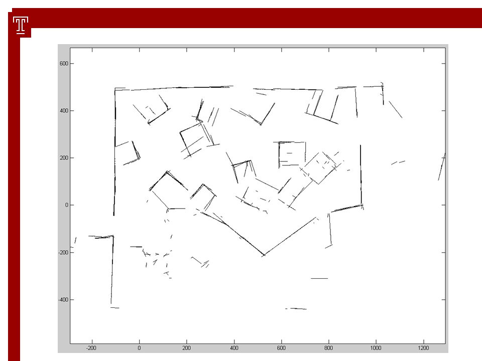
11. The following slide shows 4 example scans of a typical data set from a disaster arena set up and scanned by NIST, 2006 The entire data set consists of 64 scans, taken from 16 different positions no odometry or additional sensor data is provided No scan order is given (simulation of 16 different robots taking 4 scans each)

12. (NIST disaster data set, 4 scans out of 64)

13. The scans are superimposed on top of each other (but not merged) to gain a global map. GLOBALMAPGLOBALMAP Scans 1..n

14. A shape based algorithm resulted in a rough estimation of the robots’ poses for an initial global map

15. Results first: FFS iteratively translates/rotates the single scans to align them to a more visually consistent global map.

16. FFS problem statement: A global map is a 3n-dimensional vector defining the poses (x,y,a) of the n robots (e.g. in the NIST example we assume 64 independent robots). Given a scalar fitness target function P on the 3n dimensional space M of global maps, find vector m in M which minimizes P (P defines the quality of alignment).

17. FFS is motivated by physics: each scan is seen as a rigid body, consisting of masses (the laser reflection points). A global map is then a system of rigid bodies. Forces between the masses of the different scans create a force field. FFS simulates the movement of the bodies in this force field. FFS is a gradient descent approach. It minimizes the force field’s potential P, which resembles the visual fitness.

18. The basic principle: corresponding to the forces, scans are iteratively translated/rotated. By laws of physics, such a system converges towards a (local) minimum of its potential

19. The following questions must be answered: 1.How to design the forces, such that the overlying potential describes an appropriate fitness function for alignment 2.How to robustly design the system with respect to local minima 3.How to overcome the O(n 2 ) complexity of a brute force approach (=pair wise computation of all forces between all n scan points)

20. 1.How to design the forces, such that the overlying potential describes an appropriate fitness function for alignment

21. Design of the Force Function Goal: design force between 2 data points (laser reflection points) A correspondence V between points p1, p2 is defined as a vector: C(p1,p2) describes the strength of correspondence:

22. Strength of correspondence Gauss function of distance Mass (or weight) of points Direction of points

23. Two points p 1,p 2 correspond strongly, if… Their euclidean distance is small The influence of distance is steered by the σ t parameter of the Gauss function. Their mass (perceptual weight) is high The underlying linear structures are parallel

24. Underlying linear structures: The data is modeled using line segments The direction of a point is the direction of the closest line segment Points on parallel segments correspond strongly

25. The force acting on each point is the sum of correspondences The overlying potential is defined by with

26. FFS is a gradient descent approach to minimize this potential. FFS computes forces between points, and the resulting forces on the rigid bodies (scans). The resulting acceleration for translation, inertia and torque for rotation are computed. (These are the gradient vectors!) The resulting transformation is performed, using a dynamic step width d T.

27. A simple example: Left: initial configuration, showing forces in each data point Middle: after translation Right: after 15 iterations

28. FFS computes the transformations for all scans simultaneously. FFS does not take into account any time order of the scans, it is therefore applicable to multi robot mapping FFS can easily be changed to an online, sequential, (single robot) mapping process: each new scan is just added to the previous set of scans. To reduce computational time, the previous global map can be fixed if necessary.

29. The following questions must be answered: 1.How to design the forces such that the overlying potential describes an appropriate fitness function for alignment 2.How to robustly design the system with respect to local minima 3.How to overcome the O(n^2) complexity of a brute force approach (=pair wise computation of all forces between scan points)

30. FFS contains 2 steering parameters: 1.σT, defining the influence of distance in the force computation 1.dT, the step width of the gradient descent in each iteration.

31. Both parameters are exponentially decreasing during the iterative process. This simulates a cooling process, similar to cooling processes known from strategies like simulated annealing etc. Since σ T defines the radius of influence of data points, the process changes from global influence (large σ T ) to local influence (small σ T ). Decreasing d T allows the system to jump out of local minima in the beginning (large d T ), while allowing precise adjustment at the end (small d T )

32. Using this cooling strategy, experiments showed a very robust behavior of FFS with respect to local minima. Typically, the potential function is not monotonically decreasing, indicating escapes from possible local minima.

33. 1.How to overcome the O(n 2 ) complexity of a brute force implementation

34. The definition of the correspondence function leads to a complexity of O(n 2 ), n=number of data points if implemented straightforwardly. To reduce the complexity, different techniques can be used, taking advantage of 2 properties of the correspondence function

35. 1.For each data point, only its local neighborhood (determined by σ t ) must be examined. Techniques to reduce complexity: –KD-trees –Bounding box trees Current implementation: bounding box tree collision on the underlying line segments. Reduces complexity to an expected O(m), m = number of line segments.

36. Some numbers: NIST 2006 data set contains 21420 data points, can be modeled by 332 line segments (average: 65 points per segment) Average number of colliding segments per iteration: 1500 Computations: 65x65x1500 = 6,337,500 (compared to 21420 2 =460,000,000)

37. 1.Second complexity reduction step: Data points have to be evaluated with certain accuracy only. Approximating the force field suggests 2 techniques to reduce the complexity: –Sub sampling the linear segments, to lower the number of points (and to achieve a uniform point density!) –Fast Gauss Transform (FGT, Greengard and Strain, 1991), leading to O(n) with a constant factor depending on precision. Current implementation: resampling.

38. Some numbers: Resampling reduces the average number of data points per segment to 7 (compared to 65). The resulting number of computations is therefore 7x7x1500=73,500. Note: resampling also reduces the space complexity: only the line segments must be stored.

39. Experiments and Results 1.NIST 06 Data Set

42. Experiments and Results 2. Apartment Data Set http://staff.science.uva.nl/~zivkovic/FS2HSC/dataset.html 2000 scans taken in an apartment of size 16x8m We used every 10th scan Pre alignment based on shape

43. Initial configuration shows error (encircled) due to incorrect loop closing and is very imprecise (blurry features)

44. A large step width d T blurs the map in the first iteration steps to escape local minima

45. Iteration 50

46. Final (Iteration 150): FFS has contracted the edges and has realigned the entire map to fix the loop closing error

47. (Movie of FFS)

48. Part 1.2 Improving Sparse Laser Scan Alignment with Virtual Scans Rolf Lakaemper, Nagesh Adluru Temple University, Philadelphia,PA,USA IROS 2008

49. Problem: too little information for FFS += +=

50. Ambiguous information

51. Solution: augment laser data with hypotheses about existing objects (expected structures) : add hypotheses to the data set as if they were real data. We call the hypothetical data Virtual Scans.

52. Example 1 +=

53. Examples of expected structures

54. Real data and Virtual Scans are fed into the iterative Force Field Simulation (FFS) alignment system FFS can not distinguish between real and virtual scans After each iteration, the resulting global map is re- analyzed to state (new) hypotheses (=create VS) Real Data 1 Real Data 2 Real Data n Virtual Data … merge LLSC operation (FFS alignment) Perceived World (global map) MLSC operation (line/rectangle detection) Alignment Analysis, Create VS Intermediate result

55. Although the current (proof of concept) system can only detect simple objects (rectangles and lines), it significantly improves the performance of FFS

56. Example: rectangle detection MapMerged segmentsDetected Rectangles

57. Example: Virtual Scan (lines / rectangles)

58. Results: 1) Simulated Data Set Data Set Ground TruthAdditional Pose Error (Init Pose)

59. Results: FFS, no VS (different parameters) Sigma_0 = 30Sigma_0 = 80

60. Results: FFS &VS (Sigma_0 = 30) Iteration 10 Iteration 20 Iteration 30 Iteration 30 not showing VS

61. FFS &VS on NIST data set

62. Conclusion: Virtual Scans augment the real sensor data Virtual Scans introduce global information about expected structures Virtual Scans improve performance of FFS

63. Future Work : General: –What are reasonable structures? –Can we learn such structures? –Extend system to Multiple Hypotheses Technical: –Of course: 3D (Demo Movie)

64. PART 2 Segment Based FFS (SFFS)

65. FFS is based on computation of pair-wise interaction of LL-elements, i.e. data points. In SFFS, we keep the pair-wise computation, but performed on segments. FFS is a gradient descent approach, maximizing a potential, the ‘visual fit’. In SFFS, we keep the general gradient approach, but replace the potential with a cost that is based on segment similarity and segment merging. To compute rotation and translation of a scan in FFS, a single gradient is computed. In SFFS, we separate the two operations. FFS uses a cooling strategy to modify the gradient length SFFS determines the amount of translation and rotation solely based on the temperature level (independent of gradient length).

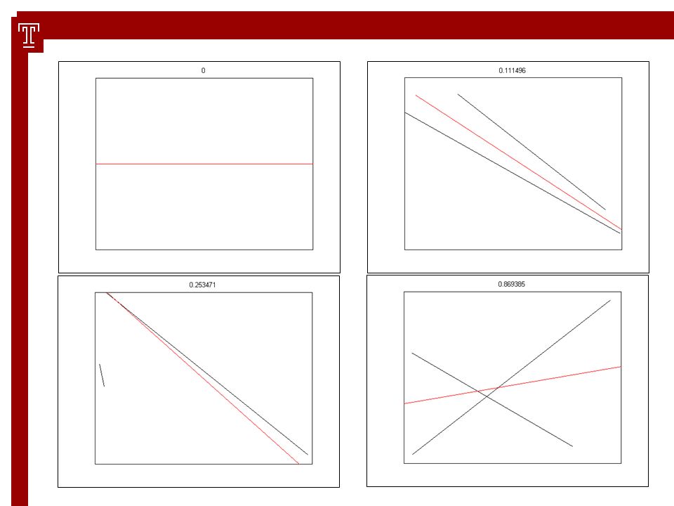
66. Segment Merging And Segment Distance Distance or Merging Cost is determined by comparison of a pair of segments to their merged version

67. Creating the Merged Segment

68. COST function takes into account: Parallelism: The greater the angles between L1 and L2 and (the target merged segment) M(L1;L2), the greater the cost of merging them together. Likewise, the angular difference of longer segments have more weight than shorter ones. Collinearity: The greater the distance of the endpoints of L1 and L2 from M, the higher the value of the cost function. Proximity: The greater the (min.) distance between L1 and L2, the higher the value of the cost function. (Details: see MATLAB function) (Note: not a metric. Already the first metric axiom is violated!)

70. Using Segment Merging in SFFS: Compute cost between all pairs of segments Cost is used as input for Gauss function to determine correspondence strength between segment pair Use correspondence strength to determine translation T and rotation A separately T and A are used as gradients for SFFS

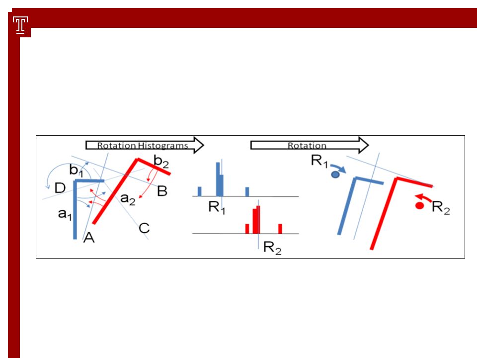
71. Rotation: In general, the strength for rotation is independent of the strength of translation. One important difference between translation and rotation of partially overlapping scans is, that, once they are rotated correctly to fit a global map, their overlapping features share the same direction (this does not hold for the position, or origin of the respective scans, which is influenced by translation). We can therefore directly compare the directions of similar features, and build a histogram of suggested rotations for best fit. For rotation, we measure the angular distance of each segment to its merged versions, as computed by the similarity measure. The optimal rotation can be computed based on these histograms (containing the correspondence strength vs. single segment rotation), using the expected values of the histogram as the resulting optimal rotation.

73. Translation: For each segment, its (soft) correspondence to all other segments is computed, along with a translation vector towards the merged version. The weighted sum of translation vectors between all pairs of segments determines the translation direction Only the direction is used, NOT the length Step width is determined by cooling process

75. Results: IT WORKS! On NIST data set: very similar result to point based system Speed gain (between the two MATLAB implementations): 50 times faster This order of magnitude is expected: Faster: segments, not points – but more expensive (constant factor!) similarity function.

76. Results: 15 scans, simultaneous SFFS

77. 20 scans from Alexander’s Texas Dataset…

78. Examples from Alexander’s Texas Dataset…trouble…

79. Map Cleaning: Segment Based Consistency Evaluation Replaces occupancy grid based systems Captures structural information Faster (operates on segments) Memory efficient Precise (no grid size needed)

80. Map Cleaning: Segment Based Consistency Evaluation 3 Steps Compute pair wise segment distance Hierarchical Clustering Evaluate Intra Cluster consistency

81. Compute pair wise segment distance Based on segment merging module. Output: n x n similarity matrix

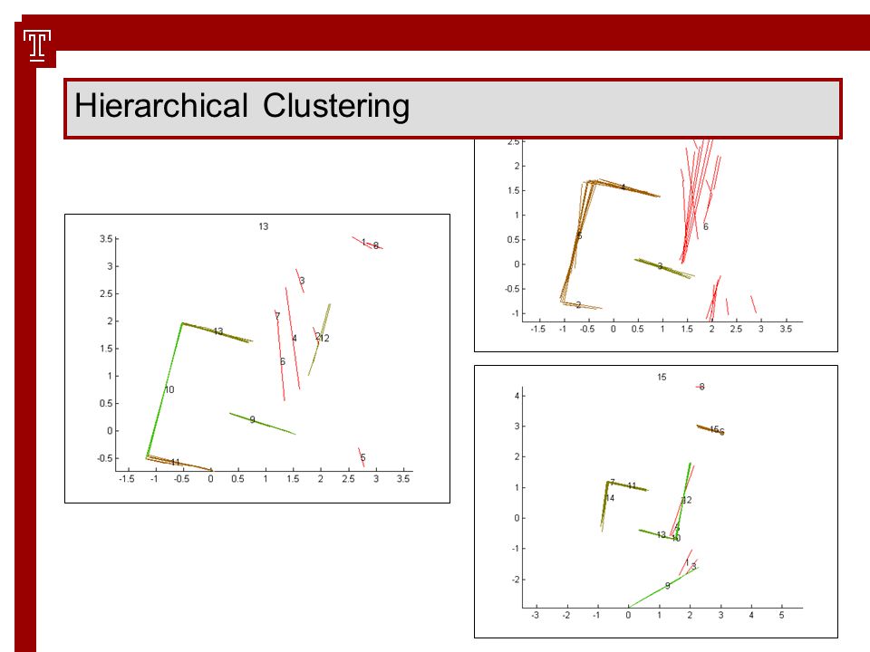
82. Hierarchical Clustering ‘Single mode’ hierarchical clustering (min. distance) Comparable to ‘connected components’ in (intuitively) segment space Bottom up: starting with each segment as single cluster, builds a hierarchy ending in a single cluster containing all segments Question: where to cut the hierarchy to obtain useful clusters? Answer: end when intra cluster distance increases significantly (standard approach)

83. Hierarchical Clustering: similarity matrix

84. Hierarchical Clustering:dendrogram

85. Hierarchical Clustering: intra cluster consistency

86. Hierarchical Clustering

90. Hierarchical Clustering, global map evaluation

91. Conclusion: Introduction of FFS, FFS + VS, SFFS (+VS) Segment based system works Segments also help in map evaluation / map cleaning THANKS!