1. Evaluation of Speaker Recognition Algorithms

2. Speaker Recognition Speech Recognition and Speaker Recognition speaker recognition performance is dependent on the channel, noise quality. Two sets of data one to enroll and the other to verify.

3. Data Collection and processing MFCC extraction Test Algorithms include AHS(Arithmetic Harmonic Sphericity) Gaussian Divergence Radial Basis Function Linear Discriminant Analysis etc.,

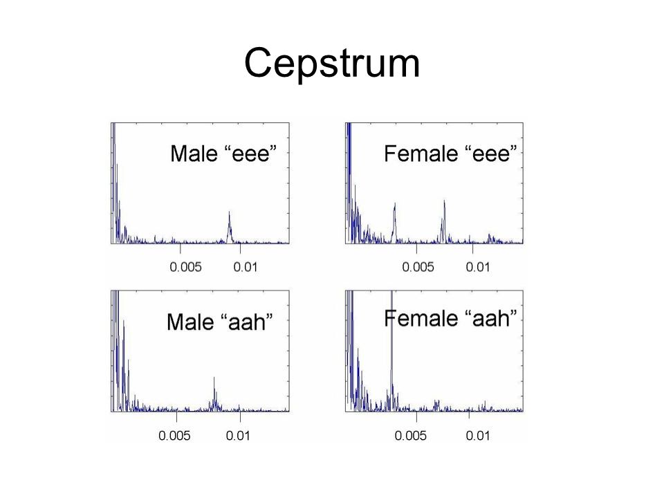
4. cepstrum Cepstrum is a common transform, used to gain information from a speech signal, whose x-axis is quefrency. Used to separate transfer function from excitation signal. X(ω)=G(ω)H(ω) log|X(ω) | =log|G(ω) | +log|H(ω) | F−1log|X(ω) | =F−1log|G(ω) | +F−1log|H(ω) |

5. Cepstrum

7. MFCC Extraction

8. Short-time FFT Frame Blocking and Windowing Eg: First Frame size=N samples Second Frame size begins M(M<N) Overlap of N-M samples and so on… Window Function: y(n)=x(n)w(n) Eg: Hamming Window: w(n)=0.54-0.46cos(2πn/N-1), 0<n<N-1

9. Mel-Frequency Wrapping Mel frequency scale is linear upto 1000Hz and logarithmic above 1000 Hz. mel(f)=2595*log(1+f / 700)

10. Mel-Spaced Filter bank

11. MFCC Cepstrum log mel spectrum back to time = MFCC MFCCs(C n ) given by where S k is the mel power spectrum coefficients

12. Arithmetic Harmonic Sphericity Function of eigen values of a test covariance matrix relative to a reference covariance matrix for speakers x and y, defined by where D is the dimensionality of the covariance matrix.

13. Gaussian Divergence Mixture of gaussian densities to model the distribution of the features of each speaker.

14. YOHO Dataset Sampling Frequency 8kHz

15. Performance – AHS with 138 subjects and 24 MFCCs

16. Performance – Gaussian Div with 138 subjects and 24 MFCCs

17. Performance – AHS with 138 subjects and 12 MFCCs

18. Performance – Gaussian Div with 138 subjects and 12 MFCCs

19. Probability Density Functions  Example 2: Review of Probability and Statistics f(x)f(x) x a=0.25 b=0.75 Probability that x is between 0.25 and 0.75 is

20. Cumulative Distribution Functions  cumulative distribution function (c.d.f.) F(x) for c.r.v. X is:  example: Review of Probability and Statistics f(x)f(x) x b=0.75 C.D.F. of f(x) is

21. Expected Values and Variance  expected (mean) value of c.r.v. X with p.d.f. f(x) is:  example 1 (discrete):  example 2 (continuous): Review of Probability and Statistics E(X) = 2·0.05+3·0.10+ … +9·0.05 = 5.35 0.05 0.25 0.20 0.15 0.10 0.15 0.05 1.02.03.04.05.06.07.08.09.0

22. Review of Probability and Statistics The Normal (Gaussian) Distribution  the p.d.f. of a normal distribution is where μ is the mean and σ is the standard deviation μ σ

23. Review of Probability and Statistics The Normal Distribution  any arbitrary p.d.f. can be constructed by summing N weighted Gaussians (mixtures of Gaussians) w1w1 w2w2 w3w3 w4w4 w5w5 w6w6

24. A Markov Model (Markov Chain) is: similar to a finite-state automata, with probabilities of transitioning from one state to another: Review of Markov Model? S1S1 S5S5 S2S2 S3S3 S4S4 0.5 0.3 0.7 0.1 0.9 0.8 0.2 transition from state to state at discrete time intervals can only be in 1 state at any given time 1.0

25. Transition Probabilities: no assumptions (full probabilistic description of system): P[q t = j | q t-1 = i, q t-2 = k, …, q 1 =m] usually use first-order Markov Model: P[q t = j | q t-1 = i] = a ij first-order assumption: transition probabilities depend only on previous state a ij obeys usual rules: sum of probabilities leaving a state = 1 (must leave a state) Review of Markov Model?

26. S1S1 S2S2 S3S3 0.5 0.3 0.7 Transition Probabilities: example: Review of Markov Model? a 11 = 0.0a 12 = 0.5a 13 = 0.5a 1Exit =0.0  =1.0 a 21 = 0.0a 22 = 0.7a 23 = 0.3a 2Exit =0.0  =1.0 a 31 = 0.0a 32 = 0.0a 33 = 0.0a 3Exit =1.0  =1.0 1.0

27. Transition Probabilities: probability distribution function: Review of Markov Model? S1S1 S2S2 S3S3 0.6 0.4 p(remain in state S 2 exactly 1 time) = 0.4 ·0.6 = 0.240 p(remain in state S 2 exactly 2 times) = 0.4 ·0.4 ·0.6 = 0.096 p(remain in state S 2 exactly 3 times) = 0.4 ·0.4 ·0.4 ·0.6 = 0.038 = exponential decay (characteristic of Markov Models)

28. Example 1: Single Fair Coin Review of Markov Model? S1S1 S2S2 0.5 S 1 corresponds to e 1 = Headsa 11 = 0.5a 12 = 0.5 S 2 corresponds to e 2 = Tailsa 21 = 0.5a 22 = 0.5 Generate events: H T H H T H T T T H H corresponds to state sequence S 1 S 2 S 1 S 1 S 2 S 1 S 2 S 2 S 2 S 1 S 1

29. Example 2: Weather Review of Markov Model? S1S1 S2S2 0.25 0.4 0.7 0.5 S3S3 0.2 0.05 0.7 0.1

30. Example 2: Weather (con’t) S 1 = event 1 = rain S 2 = event 2 = clouds A = {a ij } = S 3 = event 3 = sun what is probability of {rain, rain, rain, clouds, sun, clouds, rain}? Obs. = {r, r, r, c, s, c, r} S ={S 1, S 1, S 1, S 2, S 3, S 2, S 1 } time = {1, 2, 3, 4, 5, 6, 7} (days) = P[S 1 ] P[S 1 |S 1 ] P[S 1 |S 1 ] P[S 2 |S 1 ] P[S 3 |S 2 ] P[S 2 |S 3 ] P[S 1 |S 2 ] = 0.5 · 0.7 · 0.7 · 0.25 · 0.1 · 0.7 · 0.4 = 0.001715 Review of Markov Model? π 1 = 0.5 π 2 = 0.4 π 3 = 0.1

31. Example 2: Weather (con’t) S 1 = event 1 = rain S 2 = event 2 = clouds A = {a ij } = S 3 = event 3 = sunny what is probability of {sun, sun, sun, rain, clouds, sun, sun}? Obs. = {s, s, s, r, c, s, s} S ={S 3, S 3, S 3, S 1, S 2, S 3, S 3 } time = {1, 2, 3, 4, 5, 6, 7} (days) = P[S 3 ] P[S 3 |S 3 ] P[S 3 |S 3 ] P[S 1 |S 3 ] P[S 2 |S 1 ] P[S 3 |S 2 ] P[S 3 |S 3 ] = 0.1 · 0.1 · 0.1 · 0.2 · 0.25 · 0.1 · 0.1 = 5.0x10 -7 Review of Markov Model? π 1 = 0.5 π 2 = 0.4 π 3 = 0.1

32. Simultaneous speech and speaker recognition using hybrid architecture –Dominique Genoud, Dan Ellis, Nelson Morgan The automatic recognition process of the human voice is often divided in two part –speech recognition –speaker recognition

33. Traditional System Traditional state of the art speaker recognition system task can be divided into two parts- –Feature Extraction –Model Creation

34. Feature Extraction

35. Model Creation Once the feature is extracted, a model can be created using various techniques i.e. Gaussian Mixture Model. Once the model is created we can find distance from one model to another Based on the distance a decision can be inferred.

36. A simultaneous speaker and speech recognition A system that models the “phone” of the speaker and also the speakers features and combines them into a model could perform very well.

37. A simultaneous speaker and speech recognition Maximum a posteriori (MAP) estimation is used to generate speaker-specific models from a set of speaker independent (SI) seed models. Assuming no prior knowledge about the speaker distribution, the a posteriori probability Pr is approximated by the score defined as where the speaker-specific models for all, world model.

38. A simultaneous speaker and speech recognition In the previous equation, was determined to be 0.02 empirically. Using Viterbi algroithm, N probable speaker P(x| ) can be found. Results: –Author reported 0.7% EER compared to 5.6% EER of GMM based system on the same dataset of 100 person.

39. Speech and Speaker Combination Posteriori probabilities and Likelihoods Combination for Speech and Speaker Recognition Mohamed Faouzi BenZeghiba, Eurospeech 2003. Authors used a combination of HMM/ANN (MLP) system for this work. For the features of the speech, he used 12 MFCC coefficients with energy and their first derivatives were calculated every 10 ms over a 30 ms window.

40. System Description is the word from a set of finite word {W} is the speakers from a set of finite registered speakers {S} is ANN parameters.

41. System Description Probability that a speaker is accepted is LLR(X) is the likelihood ratio.Is GMM modelis the background model where its parameters are derived from using MAP adaptation and the world data set

42. Combination Use of MLP adaptation. –shifting the boundaries between the phone classes without strongly affecting the posterior probabilities of the speech sounds of other speakers Author proposed following formula to combine the both system

43. Combination Using posteriori on the test set it can be shown that- Probability that a speaker is accepted is Determined from a posteriori of the test set.

44. HMM-Parameter Estimation Given an observation sequence O, determine the model parameters (A,B,π) that maximize P(O|λ) where λ= (A,B,π) γ t (i) is the probability of being in state i, then

45. HMM-Parameter Estimation = Expected frequency in state i at time t=1

46. Thank You