1. Chapter 8 Image Compression

2. What is Image Compression? Reduction of the amount of data required to represent a digital image → removal of redundant data Transforming a 2-D pixel array into a statistically data set

3. Why Compression? Important in data storage data storage and data transmission data transmission Examples: – Progressive transmission of images (Internet) – Video coding. – Digital libraries and image databases – Remote sensing – Medical imaging

4. Lossless vs. Lossy Compression Compression techniques - Lossless (or information-preserving) compression: Images can be compressed and restored without any loss of information (e.g., medical imaging, satellite imaging) - Lossy compression: Perfect recovery is not possible but provides a large data compression (e.g., TV signals)

5. Data and Information Data are the means by which information is conveyed Various amounts of data may be used to represent the same amount of information Data redundancy: if n1 and n2 denote the number of information-carrying units in two data sets that represent the same information, the relative data redundancy of the first data set is

6. Redundancy In digital image compression there exist three basic data redundancies: 1. Coding redundancy 2. Spatial and Temporal redundancy 3. Irrelevant redundancy

7. Coding Redundancy Let be a discrete random variable representing the gray levels in an image Its probability is represented by Let be the total number of bits used to represent each value of The average number of bits required to represent each pixel is

8. Example: Variable-Length Coding

9. Example: Rationale behind Variable-Length Coding L avg =1.81 bits C = 4.42 R =.774

10. Spatial and Temporal Redundancy any pixel can be predicted from the value of its neighbors the information carried by individual pixels is relatively small spatial redundancy / interframe redundancy

11. Interpixel Redundancy Mapping –to reduce Spatial redundancy, image must be transformed into a more efficient format –reversible mapping vs. irreversible mapping –reversible mapping: original elements can be reconstructed from the transformed set

12. Example: Run-Length Coding Run length Pairs each pair consists of : Intensity value # pixels that have this intensity value

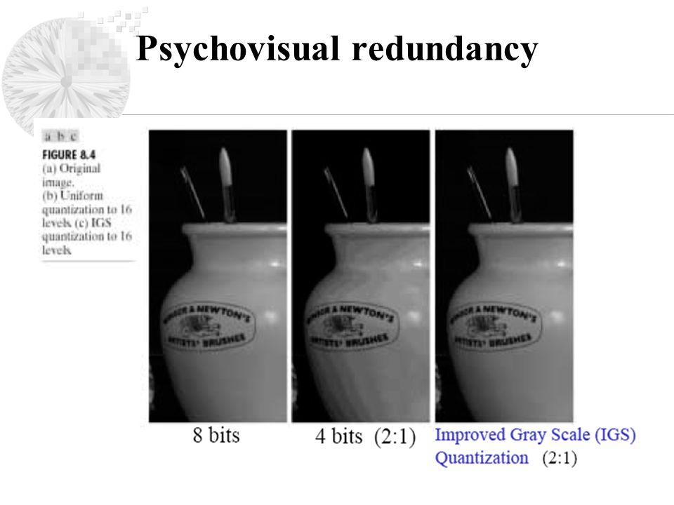
13. Psychovisual redundancy Irrelevant The eye does not respond with equal sensitivity to all visual information Certain information has less relative importance than other information in normal visual processing (psychovisually redundant) It can be eliminated without significantly impairing the quality of image perception

14. Psychovisual redundancy

16. Objective Fidelity Criteria

17. Signal-to-Noise Ratio (SNR) Mean square Signal-to-Noise ratio of the output image:

18. Subjective Fidelity Criteria Example of an absolute comparison scale:

19. Measuring Image Information A discrete source of information generates one of N possible symbols from a source alphabet set A = { }, in unit time. Example: A = {a,b c, …,z}, {0,1}, {0,1,2,..., 255 } The source output can be modeled as a discrete random variable E, which can take values in set A ={ }, with corresponding probabilities { } We will denote the symbol probabilities by the vector Naturally, The information source is characterized by the pair (A,z ).

20. Measuring Information Observing an occurrence (or realization) of the random variable E results in some gain of information denoted by I(E). This gain of information was defined to be (Shannon): The base for the logarithm depends on the units for measuring information. Usually, we use base 2, which gives the information in units of “binary digits” or “bits.” The entropy, H(z), of a source: symbol:

21. Measuring Information Higher the source entropy, higher the information associated with a source. For a fixed number of source symbols, the entropy is maximized if all the symbols are equally likely H = 1.6614 for image in figure 8.1

22. Measuring Information

23. Image Compression Models

24. Source Encoder encoder is responsible for reducing or eliminating any coding, interpixel, or psychovisual redundancy. The first block “Mapper” transforms the input data into a (usually nonvisual) format, designed to reduce interpixel (spatial) redundancy. This block is reversible and may or may not reduce the amount of data. Example: run-length encoding, image transform.

25. Source Encoder The Quantizer reduces accuracy of the mapper output in accordance with some fidelity criterion. This block reduces psychovisual redundancy and is usually not invertible. The Symbol Encoder creates a fixed or variable length codeword to represent the quantizer output and maps the output in accordance with this code. This block is reversible and reduces coding redundancy.

26. Source Decoder The decoder blocks are inverse operations of the corresponding encoder blocks (except the quantizer block, which is not invertible).

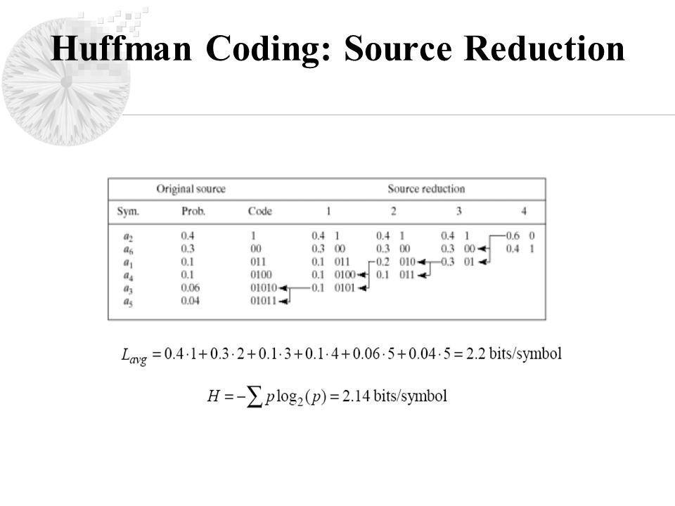
27. Huffman Coding If the symbols of an information source are coded individually, the Huffman coding yields the smallest possible number of code symbols per source symbol Method: create a series of source reductions by ordering the probabilities of the symbols under consideration and combining the lowest probability symbols into a single symbol that replace them in the next source reduction

28. Huffman Coding: Source Reduction

30. Huffman Coding: Properties The resulting code is called a Huffman code. It has some interesting properties: (1)The source symbols can be encoded (and decoded) one at time (with a lookup table). (2) It is called a block code because each source symbol is mapped into a fixed sequence of code symbols. (3) It is instantaneous because each codeword in a string of code symbols can be decoded without referencing succeeding symbols.

31. (4) It is uniquely decodable because any string of code symbols can be decoded in only one way. Huffman Coding: Properties Disadvantage: For a source with J symbols, we need J-2 source reductions. This can be computationally intensive for large J (ex. J = 256 for an image with 256 gray evels).

32. Huffman Coding: Properties Huffman coded with 7.428 bits/pixel H = 7.3838 bits/pixel C = 8/7.428 = 1.077 R = 1 – (1/1.077) = 0.0715 7.15 % coding redundancy

33. Lempel-Ziv-Welch Coding LZW coding is also an error free compression technique. Uses a dictionary Dictionary is adaptive to the data Decoder constructs the matching dictionary based on the codewords received. LZW encoder sequentially examines the image’s pixels, gray level sequences that are not in the dictionary are placed in algorithmically determined locations.

34. LZW Coding: Example Consider an example: 4 by 4, an 8-bit image The dictionary values 0-255 correspond to the pixel values 0-255. Assume a 512 word dictionary formats

35. LZW Coding: Example The image is encoded by processing its pixels in a left-to-right, top-to-down manner.

36. LZW Decoding Just like the compression algorithm, it adds a new string to the string table each time it reads in a new code. All it needs to do in addition to that is translate each incoming code into a string and send it to the output. Just like the compression algorithm, it adds a new string to the string table each time it reads in a new code. All it needs to do in addition to that is translate each incoming code into a string and send it to the output.

37. LZW Decoding: Example

38. LZW Decoding It needs to be able to take the stream of codes output from the compression algorithm, and use them to exactly recreate the input stream. One reason for the efficiency of the LZW algorithm is that it does not need to pass the sequence dictionary to the decompression code. The dictionary can be built exactly as it was during compression, using the input stream as data. Original Image = 128 bits reduced to 90 bits Disadvantages:- handling table overflow.

39. Run-Length Coding Images with repeating intensities along their rows (or columns) can often be compressed by representing the runs of identical intensities as run-length pairs. Each run-length pair specifies the start of new intensity, and the number of consecutive pixels that have that intensity. Removing spatial redundancy. Very Good for Binary Images.

40. Run-Length Coding: Approaches (1) Start position and lengths of runs of 1s for each row is used: (1,3)(7,2) (12,4) (17,2) (20,3) (5,13) (19,4) (1,3) (17,6) (2) Only lengths of runs, starting with the length of 1 run is used: 3,3,2,3,4,1,2,1,3 0,4,13,1,4 3,13,6

41. Run-Length Coding This technique is very effective in encoding binary images with large contiguous black and white regions, which would give rise to a small number of large runs of 1s and 0s. The run-lengths can in turn be encoded using a variable length code (ex. Huffman code), for further compression.

42. Run-Length Coding Let be the fraction of runs of 0s with length k. Naturally, would represent a vector of probabilities (the probability of a run of 0s being of length k). Let be the entropy associated with and be the average length of runs of 0s.

43. Run-Length Coding Let be the fraction of runs of 1s with length k. Naturally, would represent a vector of probabilities (the probability of a run of 1s being of length k). Let be the entropy associated with and be the average length of runs of 1s. The approximate run length entropy of the image is provides an estimate of the average number of bits per pixel required to code the run lengths in a binary image, using a variable-length code.

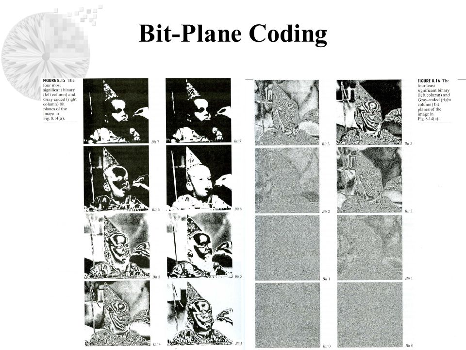
44. Bit-Plane Coding A grayscale image is decomposed into a series of binary images and each binary image is compressed by some binary compression method. This removes coding and interpixel redundancy. Given a grayscale image with gray levels, each gray value can be represented by m-bits, say, The gray value r represented by is given by the base 2 polynomial given by the base 2 polynomial This bit representation can be used to decompose the gray scale image into m binary images (bit-planes).

45. Gray Code Alternatively, one can use the m-bit Gray code to represent a given gray value. The Gray code can be obtained from by the following relationship: The Gray code of successive gray levels differ at only one position. 127 → 01111111 (binary code representation) 01000000 (Gray) 128 → 10000000 (binary code representation) 11000000 (Gray)

46. Bit-Plane Coding

48. Block Transform Coding Image transform are able to concentrate the image in a few transform coefficients. Energy packing A large number of coefficients can be discarded Transform Coding techniques operate on a reversible linear transform coefficients of the image (ex. DCT, DFT, DWT etc.)

49. Image Compression: Transform Coding Input N × N image is subdivided into subimages of size n × n n × n subimages are converted into transform arrays. This tends to pack as much information as possible in the smallest number of coefficients.

50. Image Compression: Transform Coding Quantizer selectively eliminates or coarsely quantizes the coefficients with least information. Symbol encoder uses a variable-length code to encode the quantized coefficients. Any of the above steps can be adapted to each subimage (adaptive transform coding), based on local image information, or fixed for all subimages.

51. Discrete Cosine Transform (DCT) Given a two-dimensional N by N image f (x, y), its discrete cosine transform (DCT) C(u,v) is defined as: Similarly, the inverse discrete cosine transform (IDCT) is given by

52. Discrete Cosine Transform (DCT) (1) Separable (can perform 2-D transform in terms of 1-D transform). (2) Symmetric (the operations on the variables x, y are identical) (3) Forward and inverse transforms are identical The DCT is the most popular transform for image compression algorithms like JPEG (still images), MPEG (motion pictures).

53. Transform Selection Commonly used ones are Karhunen-Loeve (Hotelling) transform (KLT), discrete cosine transform (DCT), discrete Fourier transform (DFT), discrete Wavelet transform (DWT), Walsh-Hadamard transform (WHT). Choice depends on the computational resources available and the reconstruction error that can be tolerated.

54. Transform Selection

55. Subimage Size Selection Images are subdivided into subimages of size n × n. 75% of the coefficient were truncated. Usually n =, for some integer k. This simplifies the computation of the transforms (ex. FFT algorithm). Typical block sizes used in practice are 8 × 8 and 16 × 16

56. Subimage Size Selection

57. Bit Allocation After transforming each subimage, only a fraction of the coefficients are retained. This can be done in two ways: (1) Zonal coding: Transform coefficients with large variance are retained. Same set of coefficients retained in all subimages. (2) Threshold coding: Transform coefficients with large magnitude in each subimage are retained. Different set of coefficients retained in different subimages. The retained coefficients are quantized and then encoded. The overall process of truncating, quantizing, and coding the transformed coefficients of the subimage is called bit-allocation.

58. Zonal Coding Transform coefficients with large variance carry most of the information about the image. Hence a fraction of the coefficients with the largest variance is retained

59. Threshold Coding In each subimage, the transform coefficients of largest magnitude contribute most significantly and are therefore retained. For each subimage (1)Arrange the transform coefficients in decreasing order of magnitude. (2) Keep only the top X% of the coefficients and discard rest. (3) Encode the retained coefficient using variable length code.

60. Threshold Mask & Zigzag Ordering Example

61. Normalization Matrix T(u,v) = round[T(u,v)/Z(u,v)] ^

62. Normalization Matrix

63. JPEG (Joint Photographic Experts Group) Is a compression standard for still images It defines three different coding systems: 1. A lossy baseline coding system based on DCT (adequate for most compression applications) 2. An extended coding system for greater compression, higher precision, or progressive reconstruction applications 3. A lossless independent coding system for reversible compression

64. JPEG – Baseline Coding System 1. Computing the DCT : the image is divided into 8X8 blocks; each pixel is level shifted by subtracting the quantity where is the maximum number of gray levels in the image. Then, the DCT of each block is computed. 2.Quantization : The DCT coefficients are threshold and coded using a quantization matrix, and the recorded using zig-zag scanning to form a 1-D sequence 3. Coding : The non-zero AC coefficients are Huffman coded. The DC coefficients of each block are coded relative to the DC coefficient of the previous block

65. The JPEG Standard: Baseline (1) Consider the 8x8 image (s) (2) Level shifted (s-128) (3) 2D-DCT (4) After dividing by quantization matrix qmat (5) Zigzag scan as in threshold coding.

66. Example: Implementing the JPEG Baseline Coding System

67. Example: Level Shifting

68. Example: Computing the DCT

69. Example: The Quantization Matrix

70. Example: Quantization

71. Zig-Zag Scanning of the Coefficients

72. JPEG

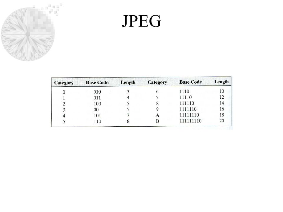
76. Example: Coding the Coefficients The DC coefficient is coded (difference between the DC coefficient of the previous block and current block) The AC coefficients are mapped to runlength pairs –(0,-26) (0,-31) ……………………..(5,-1),(0,-1),EOB These are then Huffman coded (codes are specified in the JPEG scheme)

77. Example: Decoding the Coefficients

78. Example: Denormalization

79. Example: IDCT

80. Example: Shifting Back the Coefficients

81. Example

82. Predictive Coding Does not require decomposition of grayscale image into bitplanes. Eliminate interpixel redundancy by extracting and coding only the new information in each pixel. New information in a pixel is the difference between its actual and predicted (based on “previous pixel values”) values.

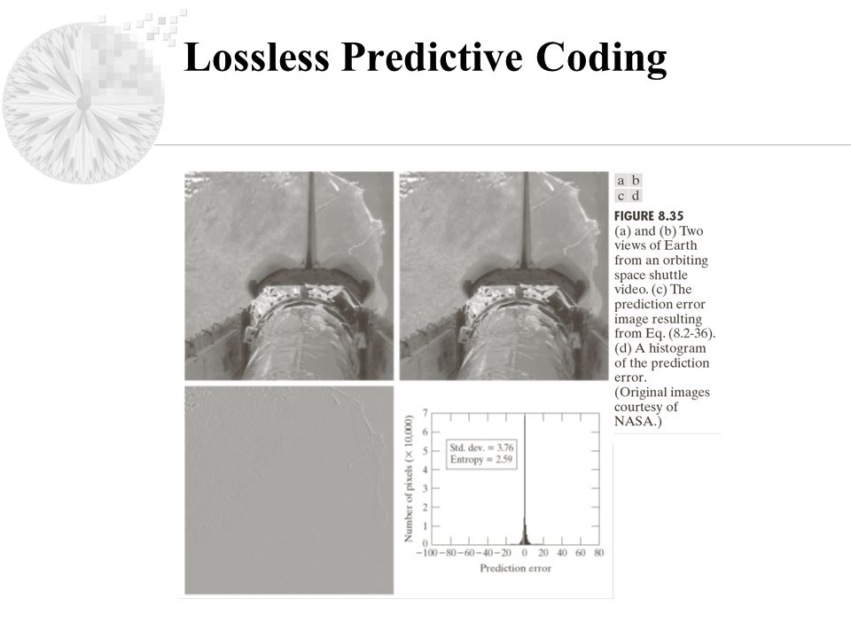
83. Lossless Predictive Coding

84. Generates an estimate of the value of a given pixel based on the values – of some past input pixels or – of some neighboring pixels (spatial prediction) Example: m=order of predictor Example: 1-D linear predictive coding

85. Lossless Predictive Coding

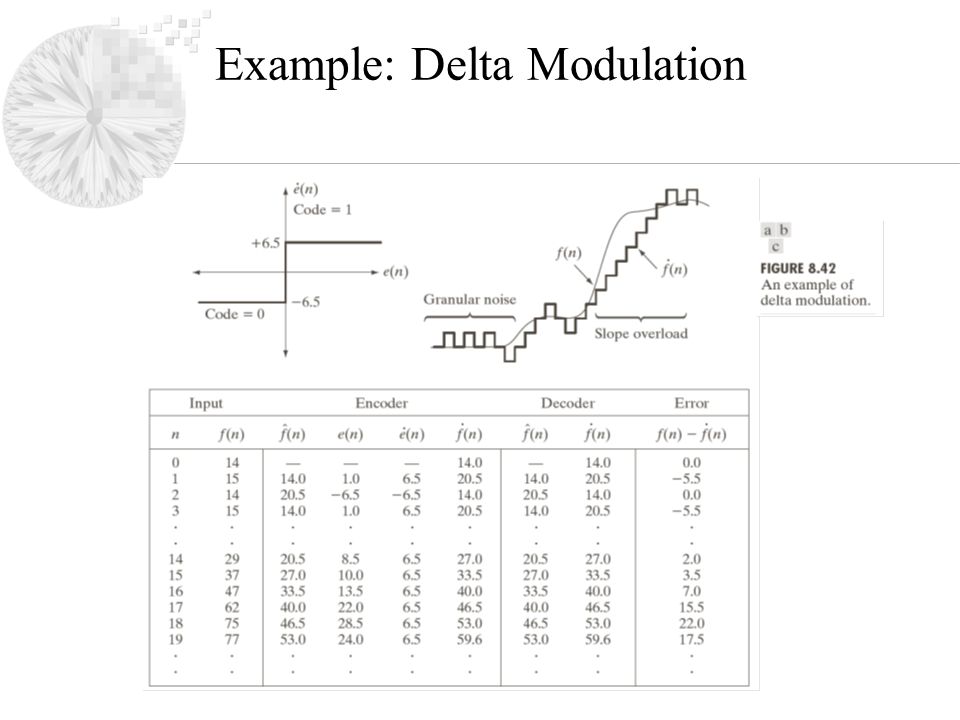
87. Lossy Predictive Coding

88. Example: Delta Modulation

90. Digital Image Watermarking Process of inserting data into an image in such a way that it can be used to make an assertion about the image. Used in: –Copyright Identification –User Identification.

91. Digital Image Watermarking Watermarks can be either visible or invisible. A visible watermark is a semi-transparent sub-image or image that is placed on top of another image(watermarked image).

92. Digital Image Watermarking Visible watermark example: f w = (1 – α)f + α w α controls the visibility of the watermark and the underlying image

93. Digital Image Watermarking Invisible watermark example: – f w = 4(f/4) + w/64

94. Digital Image Watermarking Robust invisible watermarks are designed to survive image modification (attack). Attacks: compression, filtering, rotation, cropping, ….

95. Digital Image Watermarking

96. Mark insertion:- 1.Compute the 2-D DCT of the image to be watermarked 2.Locate the K largest coeffecients, c 1, c 2, …, c k by magnitude. 3.Create a watermark by generating a K pseudo- random sequence of numbers ω 1,ω 2,…..ω k taken from a Gaussian distribution with mean = 0 and variance = 1.

97. Digital Image Watermarking 4. Embed the water mark from 3 into the k largest coeffecients from step 2 using the equation: c i - = c i.(1+ α ω i ) 1 ≤ i ≤ K 5. Compute the inverse DCT of the result obtained from step 4.

98. Digital Image Watermarking Advantages: –No obvious structure. –Embedded in a multiple frequency components. –Attacks against them tend to degrade the image.

99. Digital Image Watermarking Watermark extraction: –Compuet the 2-D DCT of the watermarked image. –Extract the K DCT coefficients c i ^ –Compute watermarks using –Measure the similarity between and γ =

100. Digital Image Watermarking D = 1 if γ ≥T 0 otherwise D = 1 indicate that watermark is present; D = 0 indicate that it was not.

101. Digital Image Watermarking