1. Dimensionality reduction: Some Assumptions High-dimensional data often lies on or near a much lower dimensional, curved manifold. A good way to represent data points is by their low-dimensional coordinates. The low-dimensional representation of the data should capture information about high- dimensional pairwise distances.

2. The basic idea of non-parameteric dimensionality reduction Represent each data-point by a point in a lower dimensional space. Choose the low-dimensional points so that they optimally represent some property of the data-points (e.g. the pairwise distances). –Many different properties have been tried. Do not insist on learning a parametric “encoding” function that maps each individual data-point to its low- dimensional representative. Do not insist on learning a parametric “decoding” function that reconstructs a data-point from its low dimensional representative.

3. Two types of dimensionality reduction Global methods assume that all pairwise distances are of equal importance. –Choose the low-D pairwise distances to fit the high-D ones (using magnitude or rank order). Local methods assume that only the local distances are reliable in high-D. –Put more weight on modeling the local distances correctly.

4. Linear methods of reducing dimensionality PCA finds the directions that have the most variance. –By representing where each datapoint is along these axes, we minimize the squared reconstruction error. –Linear autoencoders are equivalent to PCA Multi-Dimensional Scaling arranges the low- dimensional points so as to minimize the discrepancy between the pairwise distances in the original space and the pairwise distances in the low-D space.

5. Metric Multi-Dimensional Scaling Find low dimensional representatives, y, for the high- dimensional data-points, x, that preserve pairwise distances as well as possible. An obvious approach is to start with random vectors for the y’s and then perform steepest descent by following the gradient of the cost function. Since we are minimizing squared errors, maybe this has something to do with PCA? –If so, we don’t need an iterative method to find the best embedding.

6. Converting metric MDS to PCA If the data-points all lie on a hyperplane, their pairwise distances are perfectly preserved by projecting the high-dimensional coordinates onto the hyperplane. –So in that particular case, PCA is the right solution. If we “double-center” the data, metric MDS is equivalent to PCA. –Double centering means making the mean value of every row and column be zero. –But double centering can introduce spurious structure.

7. Non-linear autoencoders with extra layers are much more powerful than PCA but they can be slow to optimize and they get different, locally optimal solutions each time. Multi-Dimensional Scaling can be made non-linear by putting more importance on the small distances. A popular version is the Sammon mapping: Non-linear MDS is also slow to optimize and also gets stuck in different local optima each time. Other non-linear methods of reducing dimensionality high-D distance low-D distance

8. Problems with Sammon mapping It puts too much emphasis on getting very small distances exactly right. It produces embeddings that are circular with roughly uniform density of the map points.

9. IsoMap: Local MDS without local optima Instead of only modeling local distances, we can try to measure the distances along the manifold and then model these intrinsic distances. –The main problem is to find a robust way of measuring distances along the manifold. –If we can measure manifold distances, the global optimisation is easy: It’s just global MDS (i.e. PCA) 2-D 1-D If we measure distances along the manifold, d(1,6) > d(1,4) 1 4 6

10. How Isomap measures intrinsic distances Connect each datapoint to its K nearest neighbors in the high-dimensional space. Put the true Euclidean distance on each of these links. Then approximate the manifold distance between any pair of points as the shortest path in this “neighborhood graph”. A B

11. Using Isomap to discover the intrinsic manifold in a set of face images

12. Linear methods cannot interpolate properly between the leftmost and rightmost images in each row. This is because the interpolated images are NOT averages of the images at the two ends. Isomap does not interpolate properly either because it can only use examples from the training set. It cannot create new images. But it is better than linear methods.

13. Maps that preserve local geometry The idea is to make the local configurations of points in the low-dimensional space resemble the local configurations in the high-dimensional space. We need a coordinate-free way of representing a local configuration. If we represent a point as a weighted average of nearby points, the weights describe the local configuration.

14. Finding the optimal weights This is easy. Minimize the squared “construction” errors subject to the sum of the weights being 1. If the construction is done using less neighbors than the dimensionality of x, there will generally be some construction error –The error will be small if there are as many neighbors as the dimensionality of the underlying noisy manifold.

15. A sensible but inefficient way to use the local weights Assume a low-dimensional latent space. –Each datapoint has latent coordinates. Find a set of latent points that minimize the construction errors produced by a two-stage process: –1. First use the latent points to compute the local weights that construct from its neighbors. –2. Use those weights to construct the high- dimensional coordinates of a datapoint from the high-dimensional coordinates of its neighbors. Unfortunately, this is a hard optimization problem. –Iterative solutions are expensive because they must repeatedly measure the construction error in the high- dimensional space.

16. Local Linear Embedding: A less sensible but more efficient way to use local weights Instead of using the the latent points plus the other datapoints to construct each held-out datapoint, do it the other way around. Use the datapoints to determine the local weights, then try to construct each latent point from its neighbors. –Now the construction error is in the low-dimensional latent space. We only use the high-dimensional space once to get the local weights. –The local weights stay fixed during the optimization of the latent coordinates. –This is a much easier search.

17. The convex optimization Find the y’s that minimize the cost subject to the constraint that the y’s have unit variance on each dimension. –Why do we need to impose a constraint on the variance? fixed weights

18. The collapse problem If all of the latent points are identical, we can construct each of them perfectly as a weighted average of its neighbors. –The root cause of this problem is that we are optimizing the wrong thing. –But maybe we can fix things up by adding a constraint that prevents collapse. Insist that the latent points have unit variance on each latent dimension. –This helps a lot, but sometimes LLE can satisfy this constraint without doing what we really intend.

19. Failure modes of LLE If the neighborhood graph has several disconnected pieces, we can satisfy the unit variance constraint and still have collapses. Even if the graph is fully connected, it may be possible to collapse all the densely connected regions and satisfy the variance constraint by paying a high cost for a few outliers.

20. A typical embedding found by LLE LLE embeddings often look like this. Most of the data is close to the center of the space. A few points are far from the center to satisfy the unit variance constraint.

21. A comment on LLE It has two very attractive features –1. The only free parameters are the dimensionality of the latent space and the number of neighbors that are used to determine the local weights. –2. The optimization is convex so we don’t need multiple tries and we don’t need to fiddle with optimization parameters. It has one bad feature: –It is not optimizing the right thing! –One consequence is that it does not have any incentive to keep widely separated datapoints far apart in the low-dimensional map.

22. A probabilistic version of local MDS It is more important to get local distances right than non-local ones, but getting infinitessimal distances right is not infinitely important. –All the small distances are about equally important to model correctly. –Stochastic neighbor embedding has a probabilistic way of deciding if a pairwise distance is “local”.

23. Stochastic Neighbor Embedding First convert each high-dimensional similarity into the probability that one data point will pick the other data point as its neighbor. To evaluate a map: –Use the pairwise distances in the low- dimensional map to define the probability that a map point will pick another map point as its neighbor. –Compute the Kullback-Leibler divergence between the probabilities in the high- dimensional and low-dimensional spaces.

24. A probabilistic local method Each point in high-D has a conditional probability of picking each other point as its neighbor. The distribution over neighbors is based on the high-D pairwise distances. –If we do not have coordinates for the datapoints we can use a matrix of dissimilarities instead of pairwise distances. High-D Space i j k probability of picking j given that you start at i

25. Throwing away the raw data The probabilities that each points picks other points as its neighbor contains all of the information we are going to use for finding the manifold. –Once we have the probabilities we do not need to do any more computations in the high-dimensional space. –The input could be “dissimilarities” between pairs of datapoints instead of the locations of individual datapoints in a high-dimensional space.

26. Evaluating an arrangement of the data in a low-dimensional space Give each datapoint a location in the low- dimensional space. –Evaluate this representation by seeing how well the low-D probabilities model the high-D ones. Low-D Space i j k probability of picking j given that you start at i

27. The cost function for a low-dimensional representation For points where p ij is large and q ij is small we lose a lot. –Nearby points in high-D really want to be nearby in low-D For points where q ij is large and p ij is small we lose a little because we waste some of the probability mass in the Q i distribution. –Widely separated points in high-D have a mild preference for being widely separated in low-D.

28. The forces acting on the low-dimensional points Points are pulled towards each other if the p’s are bigger than the q’s and repelled if the q’s are bigger than the p’s i j

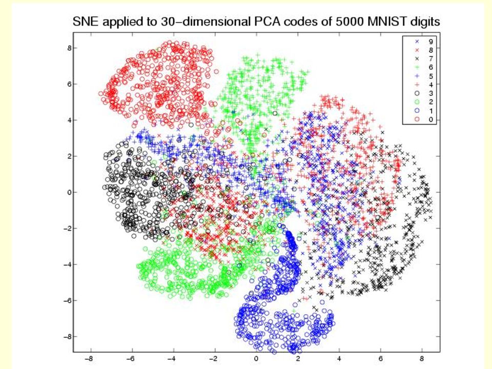
29. Data from sne paper Unsupervised SNE embedding of the digits 0-4. Not all the data is displayed

30. Picking the radius of the gaussian that is used to compute the p’s We need to use different radii in different parts of the space so that we keep the effective number of neighbors about constant. A big radius leads to a high entropy for the distribution over neighbors of i. A small radius leads to a low entropy. So decide what entropy you want and then find the radius that produces that entropy. Its easier to specify 2^entropy –This is called the perplexity –It is the effective number of neighbors.

31. Symmetric SNE There is a simpler version of SNE which seems to work about equally well. Symmetric SNE works best if we use different procedures for computing the p’s and the q’s –This destroys the nice property that if we embed in a space of the same dimension as the data, the data itself is the optimal solution.

32. Computing the p’s for symmetric SNE Each high dimensional point, i, has a conditional probability of picking each other point, j, as its neighbor. The conditional distribution over neighbors is based on the high-dimensional pairwise distances. High-D Space i j k probability of picking j given that you start at i

33. Turning conditional probabilities into pairwise probabilities To get a symmetric probability between i and j we sum the two conditional probabilities and divide by the number of points (points are not allowed to choose themselves). This ensures that all the pairwise probabilities sum to 1 so they can be treated as probabilities. joint probability of picking the pair i,j

34. Evaluating an arrangement of the points in the low- dimensional space Give each data-point a location in the low- dimensional space. –Define low-dimensional probabilities symmetrically. –Evaluate the representation by seeing how well the low-D probabilities model the high-D affinities. Low-D Space i j k

35. The cost function for a low-dimensional representation It’s a single KL instead of the sum of one KL for each datapoint.

36. The forces acting on the low-dimensional points Points are pulled towards each other if the p’s are bigger than the q’s and repelled if the q’s are bigger than the p’s –Its equivalent to having springs whose stiffnesses are set dynamically. i j extension stiffness

38. Optimization methods for SNE We get much better global organization if we use annealing. –Add Gaussian noise to the y locations after each update. –Reduce the amount of noise on each iteration. –Spend a long time at the noise level at which the global structure starts to form from the hot plasma of map points. It also helps to use momentum (especially at the end). It helps to use an adaptive global step-size.

39. t-SNE Why not use gaussians at many different spatial scales? –This sounds expensive, but if we use an infinite number of gaussians, its actually cheaper because we avoid exponentiating.

40. Optimization hacks Reputable hack: Introduce a penalty term that keeps all the map-points close together. –Then gradually relax the penalty to break symmetry slowly. Disreputable hack: Allow the probabilities to add up to 4. –This causes the map-points to curdle into small clusters leaving lots of space for clusters to move past each other. –Then make the probabilities add up to 1.

41. Two other state-of-the-art dimensionality reduction methods on the 6000 MNIST digits IsomapLocally Linear Embedding

42. t-SNE on the 6000 MNIST digits

43. The COIL20 dataset Each object is rotated about a vertical axis to produce a closed one- dimensional manifold of images.

44. Isomap & LLE for COIL20 dataset IsomapLocally Linear Embedding

45. t-SNE for COIL20 dataset

46. Using t-SNE to see what you are thinking