Download presentation
Presentation is loading. Please wait.

1
1.11.1 Functions

2
Quick Review

3
What you’ll learn about Numeric Models Algebraic Models Graphic Models The Zero Factor Property Problem Solving Grapher Failure and Hidden Behavior A Word About Proof … and why Numerical, algebraic, and graphical models provide different methods to visualize, analyze, and understand data.

4
Mathematical Model A mathematical model is a mathematical structure that approximates phenomena for the purpose of studying or predicting their behavior.

5
Numeric Model A numeric model is a kind of mathematical model in which numbers (or data) are analyzed to gain insights into phenomena.
 are analyzed to gain insights into phenomena.")
6
Algebraic Model An algebraic model uses formulas to relate variable quantities associated with the phenomena being studied.

7
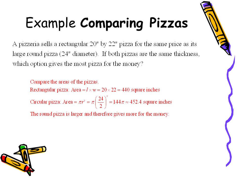
Example Comparing Pizzas

9
Graphical Model A graphical model is a visible representation of a numerical model or an algebraic model that gives insight into the relationships between variable quantities.

10
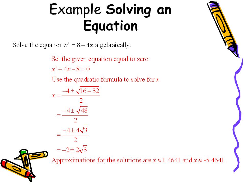
Example Solving an Equation

12
Fundamental Connection

13
Pólya’s Four Problem- Solving Steps 1. Understand the problem. 2. Devise a plan. 3. Carry out the plan. 4. Look back.

14
A Problem-Solving Process Step 1 – Understand the problem. Read the problem as stated, several times if necessary. Be sure you understand the meaning of each term used. Restate the problem in your own words. Discuss the problem with others if you can. Identify clearly the information that you need to solve the problem. Find the information you need from the given data.

15
A Problem-Solving Process Step 2 – Develop a mathematical model of the problem. Draw a picture to visualize the problem situation. It usually helps. Introduce a variable to represent the quantity you seek. Use the statement of the problem to find an equation or inequality that relates the variables you seek to quantities that you know.

16
A Problem-Solving Process Step 3 – Solve the mathematical model and support or confirm the solution. Solve algebraically using traditional algebraic models and support graphically or support numerically using a graphing utility. Solve graphically or numerically using a graphing utility and confirm algebraically using traditional algebraic methods. Solve graphically or numerically because there is no other way possible.

17
A Problem-Solving Process Step 4 – Interpret the solution in the problem setting. Translate your mathematical result into the problem setting and decide whether the result makes sense.

18
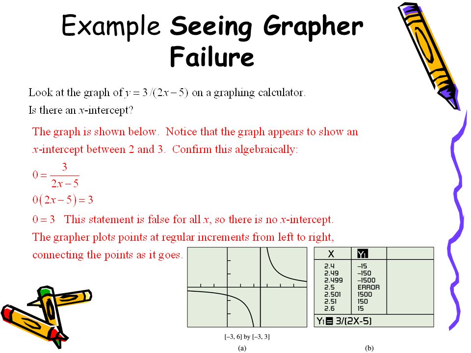
Example Seeing Grapher Failure

20
1.1(a)/1.21.1(a)/1.2 Functions and Their Properties
/1.21.1(a)/1.2 Functions and Their Properties")
21
Quick Review

22
What you’ll learn about Function Definition and Notation Domain and Range Continuity Increasing and Decreasing Functions Boundedness Local and Absolute Extrema Symmetry Asymptotes End Behavior … and why Functions and graphs form the basis for understanding The mathematics and applications you will see both in your work place and in coursework in college.

23
Function, Domain, and Range A function from a set D to a set R is a rule that assigns to every element in D a unique element in R. The set D of all input values is the domain of the function, and the set R of all output values is the range of the function.

24
Mapping

25
Example Seeing a Function Graphically

26
The graph in (c) is not the graph of a function. There are three points on the graph with x-coordinates 0.

27
Vertical Line Test A graph (set of points (x,y)) in the xy- plane defines y as a function of x if and only if no vertical line intersects the graph in more than one point.
) in the xy- plane defines y as a function of x if and only if no vertical line intersects the graph in more than one point.")
28
Agreement Unless we are dealing with a model that necessitates a restricted domain, we will assume that the domain of a function defined by an algebraic expression is the same as the domain of the algebraic expression, the implied domain. For models, we will use a domain that fits the situation, the relevant domain.

29
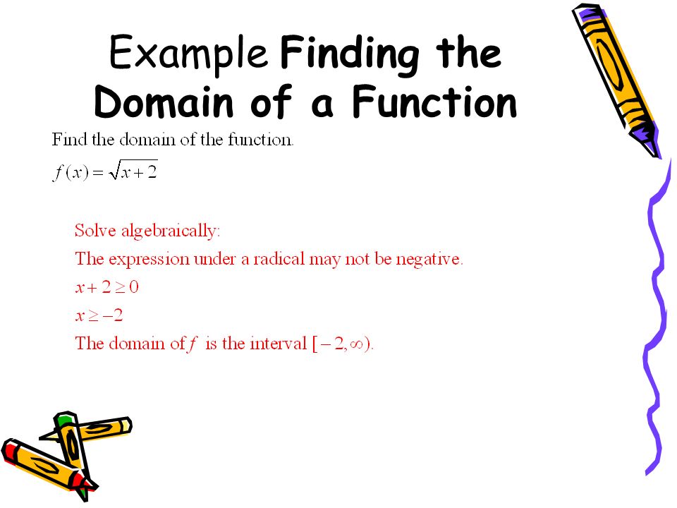
Example Finding the Domain of a Function

31
Example Finding the Range of a Function

33
Continuity

34
Example Identifying Points of Discontinuity Which of the following figures shows functions that are discontinuous at x = 2?

35
Example Identifying Points of Discontinuity Which of the following figures shows functions that are discontinuous at x = 2? The function on the right is not defined at x = 2 and can not be continuous there. This is a removable discontinuity.

36
Increasing and Decreasing Functions

37
Increasing, Decreasing, and Constant Function on an Interval A function f is increasing on an interval if, for any two points in the interval, a positive change in x results in a positive change in f(x). A function f is decreasing on an interval if, for any two points in the interval, a positive change in x results in a negative change in f(x). A function f is constant on an interval if, for any two points in the interval, a positive change in x results in a zero change in f(x).
. A function f is constant on an interval if, for any two points in the interval, a positive change in x results in a zero change in f(x)..")
38
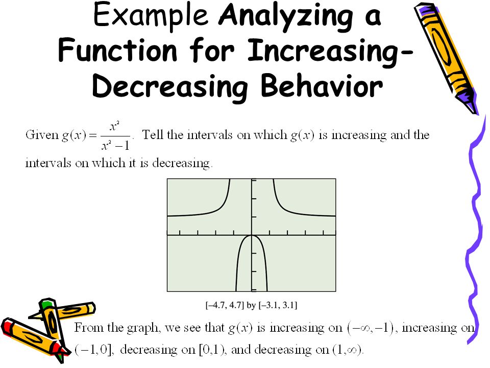
Example Analyzing a Function for Increasing- Decreasing Behavior

40
Lower Bound, Upper Bound and Bounded A function f is bounded below of there is some number b that is less than or equal to every number in the range of f. Any such number b is called a lower bound of f. A function f is bounded above of there is some number B that is greater than or equal to every number in the range of f. Any such number B is called a upper bound of f. A function f is bounded if it is bounded both above and below.

41
Local and Absolute Extrema A local maximum of a function f is a value f(c) that is greater than or equal to all range values of f on some open interval containing c. If f(c) is greater than or equal to all range values of f, then f(c) is the maximum (or absolute maximum) value of f. A local minimum of a function f is a value f(c) that is less than or equal to all range values of f on some open interval containing c. If f(c) is less than or equal to all range values of f, then f(c) is the minimum (or absolute minimum) value of f. Local extrema are also called relative extrema.
 is greater than or equal to all range values of f, then f(c) is the maximum (or absolute maximum) value of f. A local minimum of a function f is a value f(c) that is less than or equal to all range values of f on some open interval containing c. If f(c) is less than or equal to all range values of f, then f(c) is the minimum (or absolute minimum) value of f. Local extrema are also called relative extrema..")
42
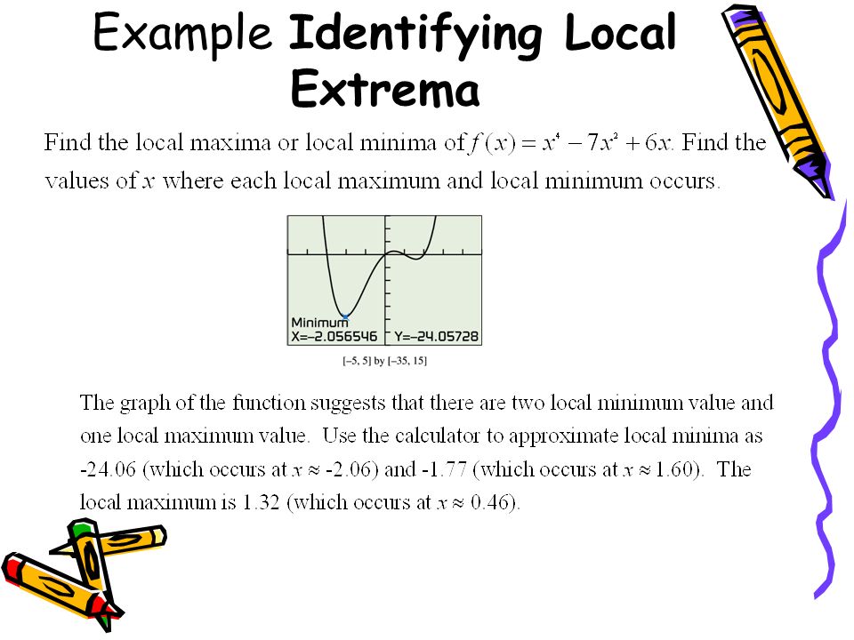
Example Identifying Local Extrema

44
Symmetry with respect to the y-axis

45
Symmetry with respect to the x-axis

46
Symmetry with respect to the origin

47
Example Checking Functions for Symmetry

49
Horizontal and Vertical Asymptotes

Similar presentations


: is all the x values Range (R): is all the y values Must write D and R in interval notation To find domain algebraically set.>")


