1. Chapter 2 : Physics & Measurement & Mathematical Review Weerachai Siripunvaraporn Department of Physics, Faculty of Science Mahidol University email&FB : wsiripun2004@hotmail.com

2. Physics Fundamental Science  Concerned with the fundamental principles of the Universe  Foundation of other physical sciences  Has simplicity of fundamental concepts Introduction CH1

3. Objectives of Physics To find the limited number of fundamental laws that govern natural phenomena To use these laws to develop theories that can predict the results of future experiments Express the laws in the language of mathematics  Mathematics provides the bridge between theory and experiment. Introduction CH1

4. Theory and Experiments Should complement each other When a discrepancy occurs, theory may be modified or new theories formulated.  A theory may apply to limited conditions. Example: Newtonian Mechanics is confined to objects traveling slowly with respect to the speed of light.  Try to develop a more general theory Introduction CH1

5. Measurements Used to describe natural phenomena Each measurement is associated with a physical quantity Need defined standards Characteristics of standards for measurements  Readily accessible  Possess some property that can be measured reliably  Must yield the same results when used by anyone anywhere  Cannot change with time CH1

6. Fundamental Quantities and Their Units

7. Quantities Used in Mechanics In mechanics, length, mass and time are used: All other quantities in mechanics can be expressed in terms of the three fundamental quantities.

8. Feel the numbers…  It is important to develop a ‘feeling’ for some of the numbers that you use. 1 kg = 1 liter of water = 1000 cc http://www.mathsisfun.com/measure/metric -length.html 1 m Duration of a heart beat when resting

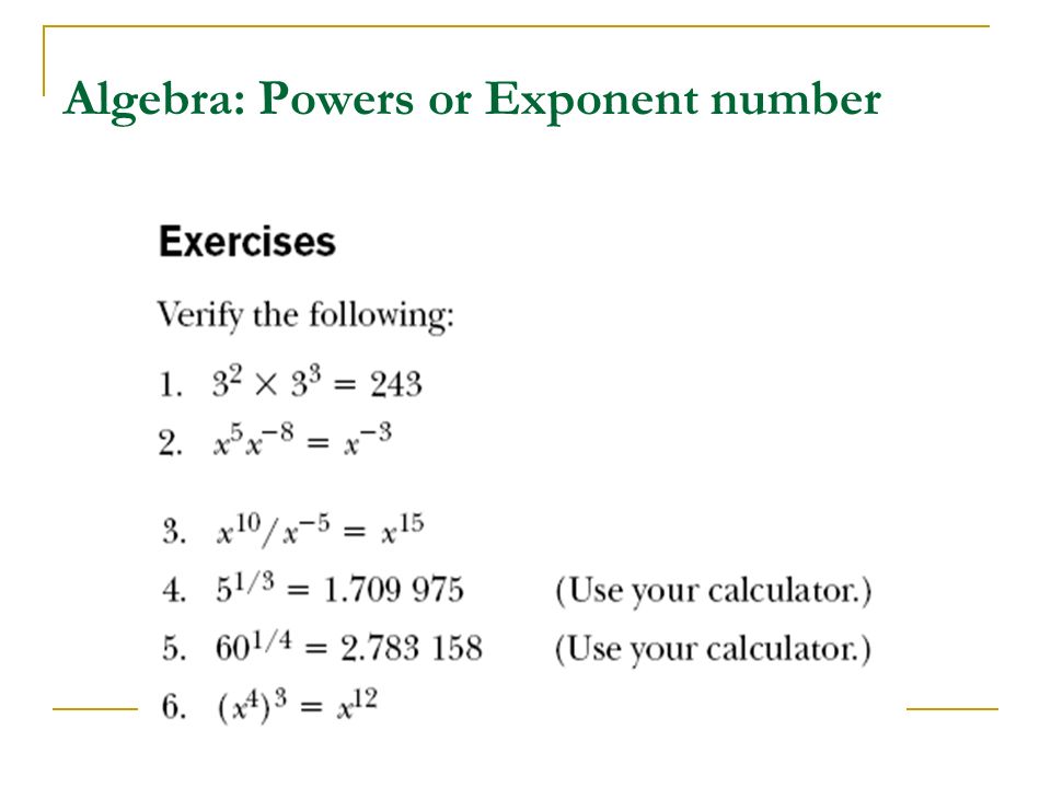
9. Prefixes Prefixes correspond to powers of 10. Each prefix has a specific name. Each prefix has a specific abbreviation. The prefixes can be used with any basic units. They are multipliers of the basic unit. Examples:  1 mm = 10 -3 m  1 mg = 10 -3 g Section 1.1 CH1

10. Prefixes, cont. Section 1.1 CH1 For example, 1 nm = 10 -9 m;3 Gs = 3 x10 9 s; 8.9 Tm = 8.9 x 10 12 m;6  g = 6 x 10 -6 g;

11. Dimensional Analysis Technique to check the correctness of an equation or to assist in deriving an equation Dimensions (length, mass, time, combinations) can be treated as algebraic quantities.  Add, subtract, multiply, divide Both sides of equation must have the same dimensions. Any relationship can be correct only if the dimensions on both sides of the equation are the same. Section 1.3 CH1

12. Dimensional Analysis, example Given the equation: x = ½ at 2 Check dimensions on each side: The T 2 ’s cancel, leaving L for the dimensions of each side.  The equation is dimensionally correct.  There are no dimensions for the constant. Section 1.3 CH1

13. Symbols The symbol used in an equation is not necessarily the symbol used for its dimension. Some quantities have one symbol used consistently.  For example, time is t virtually all the time. Some quantities have many symbols used, depending upon the specific situation.  For example, lengths may be x, y, z, r, d, h, etc. The dimensions will be given with a capitalized, non-italic letter. The algebraic symbol will be italicized. CH1

14. Conversion of Units When units are not consistent, you may need to convert to appropriate ones. Units can be treated like algebraic quantities that can cancel each other out. Always include units for every quantity, you can carry the units through the entire calculation. Section 1.4 CH1

15. Exercise Convert 1 kg/m 3 to g/cm 3 Convert 1 g/cm 3 to kg/m 3 Kinetic energy is defined as ½mv 2 and has a unit of joule (J) where m is mass in kg and v is speed in m/s. A large object has a mass about 1600 Gg and move with a speed of 0.5 km/hr. Find the kinetic energy of this object in J?

16. Objectives of Physics To find the limited number of fundamental laws that govern natural phenomena To use these laws to develop theories that can predict the results of future experiments Express the laws in the language of mathematics  Mathematics provides the bridge between theory and experiment. Introduction CH1

17. Math Review Algebra : solve basic equation, exponent number, logarithmic number, linear equation, solving simultaneous equation, etc. Scientific Notations. Trigonometry and Geometry Vector Calculus : Derivative and Integration

18. Scientific Notation For very large and very small number, it becomes cumbersome to read, write and memorize. How would you describe these numbers? 70,000,000,000,000,000,000,000,000,000,000,000,000,000,000,00 0,000,000,000,000,000,000.00 and 0.0000000000000000000000000000000000000000000000000000 00000000000000000000000000000000000000000000000000000 00000000000000000000000000000000000000000000000000000 000000000000001

19. Scientific Notation For very large and very small number, it becomes cumbersome to read, write and memorize. We avoid this problem by using a method dealing with powers of 10. Number of zeros

20. Scientific Notation Numbers expressed as some power of 10 multiplied by another number between 1 and 10 are said to be in scientific notation.

21. Calculus There are two components to calculus. One is the measure the rate of change at any given point on a curve. This rate of change is called the derivative. The second part is used to measure the exact area under a curve. This is called the integral. The derivative and the integral are inverse functions of each other. http://www.wtv-zone.com/Angelaruth49/Calculus.html

22. Calculus: Derivative To measure the rate of change of  x is to calculate the slope slope = y 2 -y 1 =  y x 2 -x 1  x When  x → 0,it become a measurement of the rate of change at any given point on a curve, or “the derivative”.

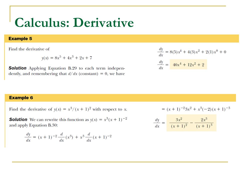
23. Calculus: Derivative

25. Exercise Find the derivative of y(x), where 1. y(x) = x 3 + 5x/(x+1) 2. y(x) = Asin(5x) + Bcos(wx) where A, B and w are constant. 3. y(x) = x 2 cos(x 2 ) 4. Find the derivative of y = f(x) = x 2 + 3x with respect to x = x 0. Use this to find the value of the derivative at (a) x 0 = 2 and (b) x 0 = -4. 5. (a) y = x 2 + 3x + 3; find dy/dx; (b) y = (x-5) 2 ; find dy/dx and d 2 y/dx 2. 6. (a) y = (3-2x)/(3+2x), find dy/dx; (b) y = 1/x, find dy/dx and d 2 y/dx 2.

26. Calculus : Integration Integration is the measure of the area under a curve and an inverse of the derivative. Integration from x 1 to x 2 is equal to the area under a curve ≈  x ½ (y 2 +y 1 ) When  x → 0,it become an area under a curve at any given point on a curve, or “the integration”.

27. Calculus : Integration

28. In physics, the students in fact need to know how to do calculus. However, in this course, we try to minimize the use of calculus or only require “simple” calculus.

29. Vectors Vector quantities  Physical quantities that have both numerical and directional properties Mathematical operations of vectors in this chapter  Addition  Subtraction Coordinate Systems used to describe the position of a point in space  Cartesian coordinate system  Polar coordinate system CH3

30. Cartesian Coordinate System Also called rectangular coordinate system x- and y- axes intersect at the origin Points are labeled (x,y) Polar Coordinate System Origin and reference line are noted Point is distance r from the origin in the direction of angle , ccw from reference line  The reference line is often the x-axis. Points are labeled (r,  ) CH3

31. Polar to Cartesian Coordinates & Cartesian to Polar Coordinates Based on forming a right triangle from r and  x = r cos  y = r sin  If the Cartesian coordinates are known: Section 3.1 CH3

32. Example 3.1 The Cartesian coordinates of a point in the xy plane are (x,y) = (-3.50, -2.50) m, as shown in the figure. Find the polar coordinates of this point. Solution: From Equation 3.4, and from Equation 3.3, Section 3.1 CH3 Convert r and  to x and y?

33. Vectors and Scalars A scalar quantity is completely specified by a single value with an appropriate unit and has no direction.  Many are always positive  Some may be positive or negative  Rules for ordinary arithmetic are used to manipulate scalar quantities. A vector quantity is completely described by a number and appropriate units (called magnitude) plus a direction. Section 3.2 CH3

34. Vector Example A particle travels from A to B along the path shown by the broken line.  This is the distance traveled and is a scalar. The displacement is the solid line from A to B  The displacement is independent of the path taken between the two points.  Displacement is a vector. Section 3.2 Force is a good example of vector quantity. CH3

35. Vector Notation Text uses bold with arrow to denote a vector: Also used for printing is simple bold print: A When dealing with just the magnitude of a vector in print, an italic letter will be used: A or | |  The magnitude of the vector has physical units.  The magnitude of a vector is always a positive number. When handwritten, use an arrow: CH3 Magnitudes are always positive! A vector can never equal a scalar. Never write

36. Remember, vectors have both magnitude and direction. You can specify a vector by:  magnitude and direction (5 meters, northeast)  magnitude and angle it makes with some axis (5 meters, 45  counterclockwise from +x axis)  components with respect to axes. If a problem requires a vector as an answer, your answer must provide information about both a magnitude and a direction. Vector Notation

37. Equality of Two Vectors Two vectors are equal if they have the same magnitude and the same direction. if A = B and they point along parallel lines All of the vectors shown are equal. Allows a vector to be moved to a position parallel to itself Section 3.3 CH3

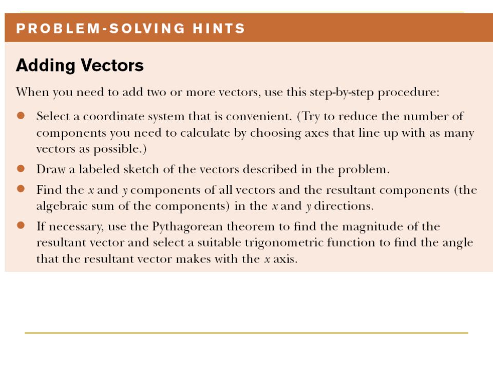
38. Adding Vectors Vector addition is very different from adding scalar quantities. When adding vectors, their directions must be taken into account. Units must be the same Graphical Methods  Use scale drawings Algebraic Methods  More convenient Section 3.3 CH3

39. Adding Vectors Graphically Choose a scale. Draw the first vector,, with the appropriate length and in the direction specified, with respect to a coordinate system. Draw the next vector with the appropriate length and in the direction specified, with respect to a coordinate system whose origin is the end of vector and parallel to the coordinate system used for. Section 3.3 CH3

40. Tip (or Head) to Tail Method for Adding Two Vectors Place the tail of the second vector at the tip of the first vector. The resultant is the vector from the beginning tail to the ending tip. A B A BA+B A “Slide” vector B so that its tail touches A’s tip. B The resultant is drawn from the origin of the first vector to the end of the last vector. Measure the length of the resultant and its angle.  Use the scale factor to convert length to actual magnitude. Ref?

41. Parallelogram Method for Adding Two Vectors The tail of the second vector is placed at the tail of the first vector. The two vectors define a parallelogram. The resultant is the vector along the diagonal of the parallelogram. A B A+B A “Slide” vector B so that its tail touches A’s tail. A B Complete the parallel- ogram. The resultant is the diagonal. B The resultant is drawn from the origin of the first vector to the end of the last vector. Measure the length of the resultant and its angle.  Use the scale factor to convert length to actual magnitude. Ref?

42. Both the tip to tail and parallelogram method produce the same resultant. A B A+B A B The magnitude of the sum is always less than or equal to the sum of the magnitudes of the vectors being added; this may provide clues to incorrectly worked problems. Ref?

43. What do you think of this: A B 1 A+B A B 3 A B 2 BAD! WRONG! DO NOT TRY THIS AT HOME! (or in class, either) You never saw that done here! Ref?

44. Adding Vectors Graphically, final When you have many vectors, just keep repeating the process until all are included. The resultant is still drawn from the tail of the first vector to the tip of the last vector. Section 3.3 CH3

45. Adding Vectors, Rules When two vectors are added, the sum is independent of the order of the addition.  This is the Commutative Law of Addition. Section 3.3 CH3

46. Adding Vectors, Rules cont. When adding three or more vectors, their sum is independent of the way in which the individual vectors are grouped.  This is called the Associative Property of Addition. Section 3.3 CH3

47. Adding Vectors, Rules final When adding vectors, all of the vectors must have the same units. All of the vectors must be of the same type of quantity.  For example, you cannot add a displacement to a velocity. Section 3.3 CH3

48. Negative of a Vector The negative of a vector is defined as the vector that, when added to the original vector, gives a resultant of zero.  Represented as  The negative of the vector will have the same magnitude, but point in the opposite direction. Section 3.3 CH3

49. Subtracting Vectors Special case of vector addition: If, then use Continue with standard vector addition procedure. Section 3.3 CH3

50. Subtracting Vectors, Method 2 Another way to look at subtraction is to find the vector that, added to the second vector gives you the first vector.  As shown, the resultant vector points from the tip of the second to the tip of the first. Section 3.3 CH3

51. Vector Multiplication by a Scalar If a is a scalar then is a vector parallel to and a times the length of. B C = 2 B C = 0.5 B C = -2 B can be longer than (if a>1) or shorter than (if a<1). If a is negative, then is in the opposite direction to. Ref?

52. Multiplying or Dividing a Vector by a Scalar The result of the multiplication or division of a vector by a scalar is a vector. The magnitude of the vector is multiplied or divided by the scalar. If the scalar is positive, the direction of the result is the same as of the original vector. If the scalar is negative, the direction of the result is opposite that of the original vector. Section 3.3 CH3

53. Component Method of Adding Vectors Graphical addition is not recommended when:  High accuracy is required  If you have a three-dimensional problem Component method is an alternative method  It uses projections of vectors along coordinate axes Section 3.4 CH3

54. Components of a Vector A component is a projection of a vector along an axis.  Any vector can be completely described by its components. It is useful to use rectangular components.  These are the projections of the vector along the x- and y- axes. Section 3.4 CH3 are the component vectors of.  They are vectors and follow all the rules for vectors. A x and A y are scalars, and will be referred to as the components of.

55. Components of a Vector Assume you are given a vector It can be expressed in terms of two other vectors, and These three vectors form a right triangle. Section 3.4 The y-component is moved to the end of the x-component. This is due to the fact that any vector can be moved parallel to itself without being affected.  This completes the triangle. CH3

56. Components of a Vector The x-component of a vector is the projection along the x-axis. The y-component of a vector is the projection along the y-axis. This assumes the angle θ is measured with respect to the x- axis. Section 3.4 The components are the legs of the right triangle whose hypotenuse is the length of A.   May still have to find θ with respect to the positive x-axis CH3

57. Components of a Vector, final The components can be positive or negative and will have the same units as the original vector. The signs of the components will depend on the angle. Section 3.4 CH3

58. Unit Vectors A unit vector is a dimensionless vector with a magnitude of exactly 1. Unit vectors are used to specify a direction and have no other physical significance. Section 3.4 The symbols represent unit vectors They form a set of mutually perpendicular vectors in a right-handed coordinate system The magnitude of each unit vector is 1 CH3

59. Unit Vectors in Vector Notation A x is the same as A x and A y is the same as A y etc. The complete vector can be expressed as: Section 3.4 CH3

60. Position Vector, Example A point lies in the xy plane and has Cartesian coordinates of (x, y). The point can be specified by the position vector. This gives the components of the vector and its coordinates. Section 3.4 CH3

61. Adding Vectors Using Unit Vectors Using Then So R x = A x + B x and R y = A y + B y Section 3.4 CH3

62. y x

64. Example 3.5 – Taking a Hike A hiker begins a trip by first walking 25.0 km southeast from her car. She stops and sets up her tent for the night. On the second day, she walks 40.0 km in a direction 60.0° north of east, at which point she discovers a forest ranger’s tower. Section 3.4 CH3

65. Example 3.5 – Solution, Finalize The resultant vector has a magnitude of 41.3 km and is directed 24.1° north of east. The units of are km, which is reasonable for a displacement. From the graphical representation, estimate that the final position of the hiker is at about (38 km, 17 km) which is consistent with the components of the resultant. Section 3.4

66. Adding Vectors by using unit vectors is a vector 66.0 units long at a 28  angle with respect to the positive x axis. is a vector 40.0 units long at a 56  angle with respect to the negative x axis. Calculate and give the resultant in terms of its (a) components and (b) magnitude and angle with the x axis. = (A x + B x ) î + (A y + B y ) ĵ = (58.27 + -22.37) î + (30.99 + 33.16) ĵ = 35.9 î + 64.1 ĵ A x = A cos  = 66.0 cos 28.0  = 58.27 B x = - B cos  = - 40.0 cos 56  = - 22.37 A y = A sin  = 66.0 sin 28.0  = 30.99 B y = B sin  = 40.0 sin 56  = 33.16 C x = 35.9 C y = 64.1

68. Vector Multiplications Dot product Cross product (will be later discussed when used)

69. Dot Product Using in Work,Power, Electric flux, Electrical potential energy, etc. Properties of dot product 0  ≤  0  = 90  : A  B = 0 90  <  ≤ 180  : A  B < 0

70. Dot Product In Unit vector form In special case:

71. Cross Product Direction of C is perpendicul ar to AB plane Using in Torque, angular momentum, magnetic force, magnetic field, etc.

72. Cross Product Properties: 1. 2. 3. 4. 5.

73. Cross Product In Unit vector form:

74. Vector calculus Derivative of r w.r.t time is

75. I am skipping the rest of these slides, but you should review by yourself to make sure you can do the math!. Math is important in learning Physics!

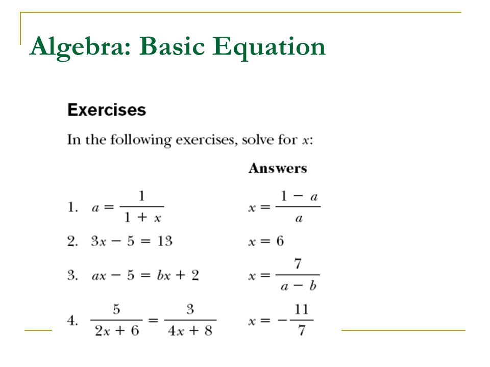
76. Algebra: Basic Equation An equation is a statement of equality, i.e. both sides of the equation are equal. Some equations contain unknown variables, such as x, either on the left side or right side or both. We must solve for its value which still make the statement correct. Example 2.1.1: Solve 5x – 10 = 20. Example 2.1.2: Find a from 5/(a+2) = 3/(a-2). In all cases, whatever operation is performed on the left side of the equality must also be performed on the right side.

77. Algebra: Basic Equation

79. Algebra: Powers or Exponent number

81. Algebra: Factoring x 2 + 6x + 9 = (x + 3) 2 x 2 – 6x + 9 = (x – 3) 2 x 2 – 16 = (x + 4)(x – 4)

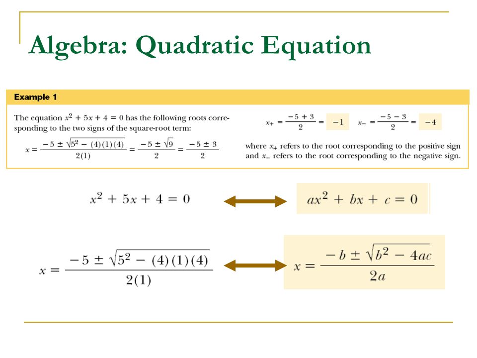
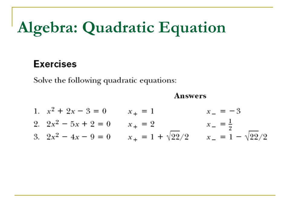
82. Algebra: Quadratic Equation

85. Algebra: Linear Equation

86. If m > 0, the straight line has a positive slope. If m < 0, the straight line has a negative slope.

87. Algebra: Linear Equation

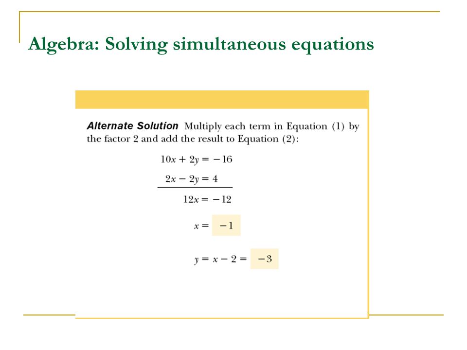
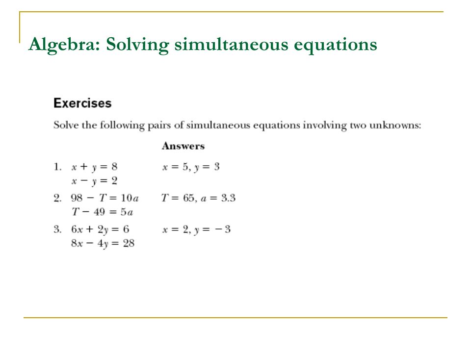
88. Algebra: Solving simultaneous equations If a problem has two unknowns, a unique solution is possible only if we have two equations. In general, if a problem has n unknowns, its solution requires n equations. In order to solve two simultaneous equations involving two unknowns, x and y, we solve one of the equations for x in terms of y and substitute this expression into the other equation. This equation has two unknown, x and y. Such an equation does not have a unique solution. For example, x = 0 and y = 3 is a solution for this equation. x = 5 and y = 0 is also a solution. x= 2 and y = 9/5 is also another solution.

89. Algebra: Solving simultaneous equations

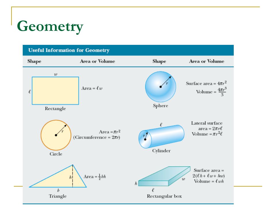
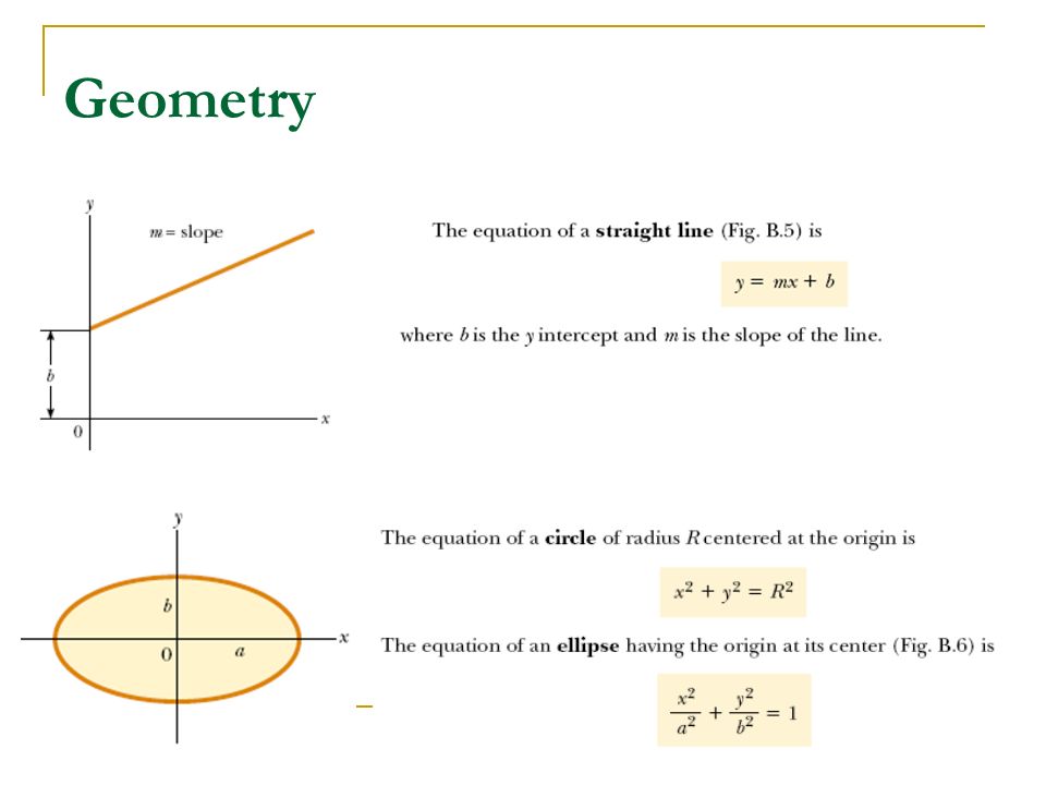
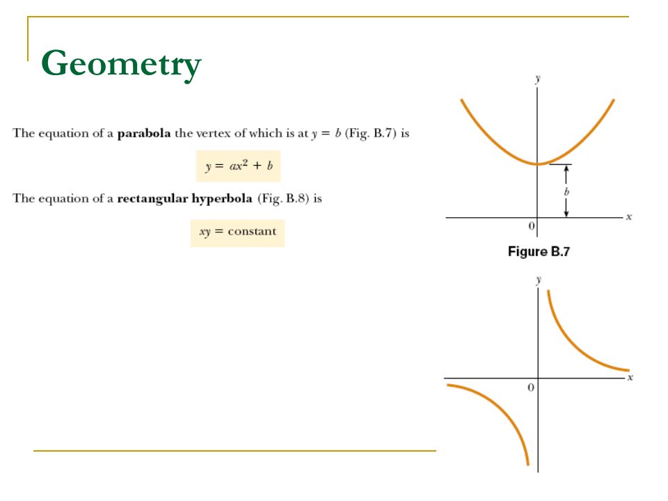
92. Geometry

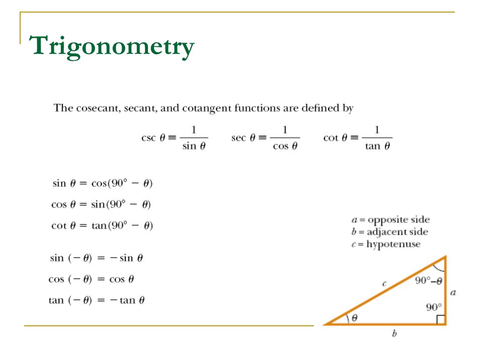
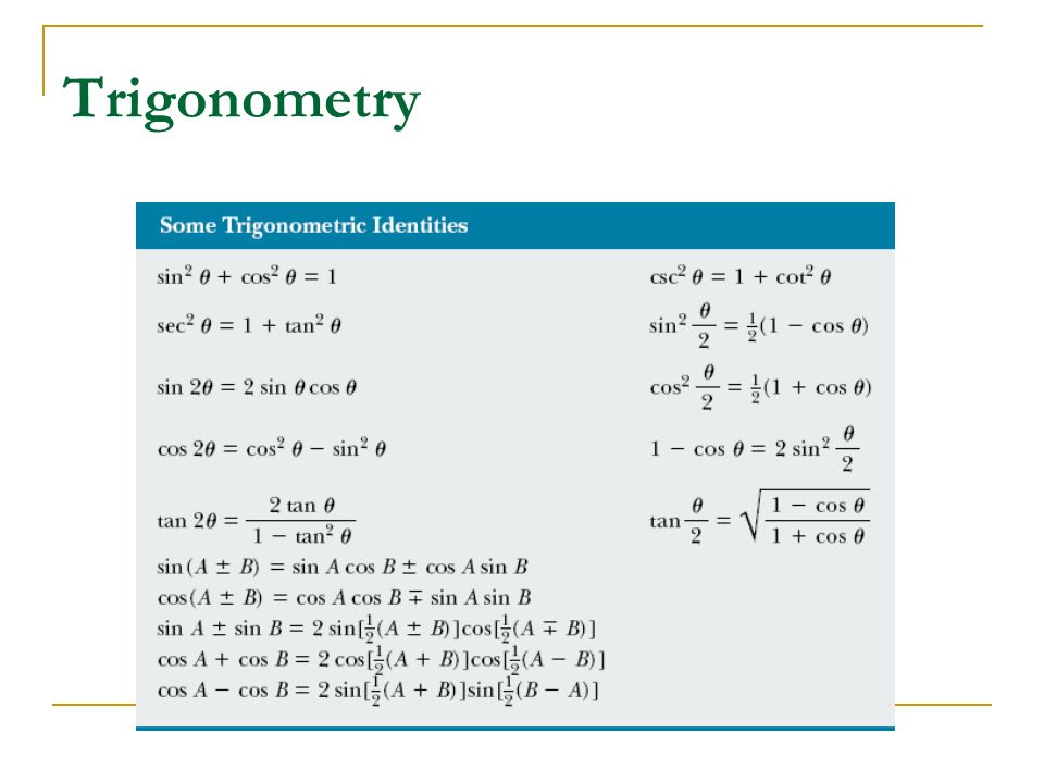
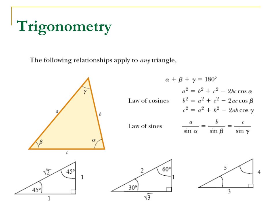
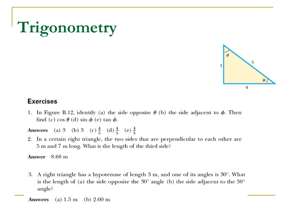
96. Trigonometry