1. Practical Statistical Analysis Objectives: Conceptually understand the following for both linear and nonlinear models: 1.Best fit to model parameters 2.Experimental error and its estimate 3.Prediction confidence intervals 4.Single-point confidence intervals 5.Parameter confidence intervals 6.Experimental design Larry Baxter ChEn 477

2. Linear vs. Nonlinear Models Linear and nonlinear refer to the coefficients, not the forms of the independent variable. The derivative of a linear model with respect to a parameter does not depend on any parameters. The derivative of a nonlinear model with respect to a parameter depends on one or more of the parameters.

3. Linear vs. Nonlinear Models

4. Typical Data

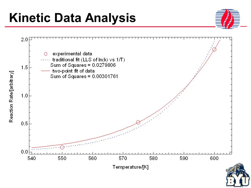
5. Kinetic Data Analysis

7. Graphical Summary The linear and non-linear analyses are compared to the original data both as k vs. T and as ln(k) vs. 1/T. As seen in the upper graph, the linearized analysis fits the low-temperature data well, at the cost of poorer fits of high temperature results. The non- linear analysis does a more uniform job of distributing the lack of fit. As seen in the lower graph, the linearized analysis evenly distributes errors in log space

8. A practical Illustration

9. Extension

10. For Parameter Estimates In all cases, fit what you measure, or more specifically the data that have normally distributed errors, rather than some transformation of this. Any nonlinear transformation (something other than adding or multiplying by a constant) changes the error distribution and invalidates much of the statistical theory behind the analysis. Standard packages are widely available for linear equations. Nonlinear analyses should be done on raw data (or data with normally distributed errors) and will require iteration, which Excel and other programs can handle.

11. Two typical datasets

12. Straight-line Regression EstimateStd Errort-StatisticP-Value intercept0.2393963.3021e-372.49779.13934e-14 slope-3.264e-41.0284e-5-31.73491.50394e-10 EstimateStd Errort-StatisticP-Value intercept0.2410011.733e-4139.0413.6504e-10 slope-3.214e-45.525e-6-58.17392.8398e-8

13. Mean Prediction Bands

14. Single-Point Prediction Bands

15. Point and Mean Prediction Bands

16. Rigorous vs. Propagation of Error

17. Propagation of Error

18. Single-Point Prediction Band

19. Residual SP Prediction Band (95%)

20. Prediction Band Characteristics

22. Nonlinear Equations

23. Parameter Characteristics Linear models Parameters are explicit functions of data – do not depend on themselves. Parameters require no iteration to compute. Normal equations are independent of parameters. Nonlinear models Parameters depend on themselves – need an estimate to begin iterative computation Parameters generally determined by converging and optimization problem, not by explicit computation. Optimization problem commonly quite difficult to converge.

24. ANOVA and Conf. Int. Tables DFSSMSF-StatisticP-Value x12.8515e-4 1007.11.50394e-10 Error92.5483e-62.83142e-7 Total102.8770e-4 DFSSMSF-Statistic P-Value x12.89221e-4 3384.212.8398e-8 Error54.27311e-78.54621e-8 Total62.89649e-4 EstimateStandard ErrorConfidence Interval intercept0.2393960.00330212{0.231926,0.246866} slope-3.26366e-41.02841e-5{-3.49631e-4,-3.03102e-4} EstimateStandard ErrorConfidence Interval intercept0.2410010.00173331{0.236545,0.245457} slope-3.2139e-45.52469e-6{-3.35595e-4,-3.07191e-4}

25. Confidence Interval Ranges

26. Some Interpretation Traps It would be easy, but incorrect, to conclude That reasonable estimates of the line can, within 95% probability, be computed by any combination of parameters within the 95% confidence interval for each parameter That experiments that overlap represent the same experimental results, within 95% confidence That parameters with completely overlapped confidence intervals represent essentially indistinguishable results If you consider the first graph in this case, all of these conclusions seem intuitively incorrect, but experimenters commonly draw these types of conclusions. Joint or simultaneous confidence regions (SCR) address these problems

27. Simultaneous Confidence Region

28. Regions and Intervals Compared

29. Nonlinear SCR More Complex The Cauchy or Lorentz equation (is a probability density function and describes some laser line widths). In this case, there are 4 noncontiguous regions.

30. Sim. or Joint Conf. Regions Region defined by

31. Simultaneous Confidence Regions Overlapping confidence intervals is a poor test for difference in data sets. Data that may appear to be similar based on confidence intervals may in fact be quite different and certainly distinct from one another. Parameters in the lonely corners of interval unions are exceptionally poor estimates.

32. Confidence Region Characteristics

33. Nonlinear Equations Regions assume many shapes and may not be contiguous. Parameters generally correlated, but not linearly correlated. Parameter uncertainty usually much smaller than confidence interval at given values of other parameters. Parameter uncertainty range exceeds conf. interval range and may not be bounded.

34. Experimental Design In this context, experimental design means selecting the conditions that will maximize the accuracy of your model for a fixed number of experiments. There are many experimental designs, depending on whether you want to maximize accuracy of prediction band, all parameters simultaneously, a subset of the parameters, etc. The d-optimal design maximizes the accuracy of all parameters and is quite close to best designs for other criteria. It is, therefore, by far the most widely used.

35. Fit vs. Parameter Precision y x Generally there is a compromise between minimizing parameter variance and validating the model. Four ways of using 16 experiments Design 1234 Lack of fit df 02214 Pure error df 1412 0 0.250.280.340.41 P sites24416 1 2 3 4

36. Typical (nonlinear) Application

37. Example Point No. 10.10.06380.10.06380.9540.5833 0.03150 20.20.18700.60.45690.9540.6203 -0.00550 30.30.24951.10.65740.9540.6049 0.00990 40.40.32071.60.78910.9540.6056 0.00920 50.50.33562.10.81970.9540.5567 0.05810 60.60.50402.60.97864.6051.0428 -0.05280 70.70.50303.10.95454.6050.9896 0.00040 80.80.64213.61.04614.6051.0634 -0.07340 90.90.64124.11.03124.6051.0377 -0.04770 101.00.56784.60.92564.6050.9257 0.06430 Compare 3 different design, each with the same number of data points and the same errors

38. SCR Results for 3 Cases 10 points equally spaced where Y changes fastest (0-1) 10 equally spaced points between 0 and 4.6 Optimal design (5 pts at 0.95 and 5 pts at 4.6)

39. Prediction and SP Conf. Intervals

40. Improved Prediction & SP Intervals Optimal design (blue) improves predictions everywhere, including extrapolated regions. Recall data for optimal design regression were all at two points, 0.95 and 4.6.

41. Linear Design Summary For linear systems with a possible experimental range from x 1 to x 2 Straight line – equal number of points at each of two extreme points Quadratic – extreme points plus middle Cubic – extreme points plus points that are located at In general, the optimal points are at the maxima of Generally, a few points should be added between two of these points to assure goodness of fit. (equally spaced would be at)

42. Nonlinear Experimental Design

43. Nonlinear Design Summary

44. Analytical and Graphical Solutions

45. Conclusions Statistics is the primary means of inductive logic in the technical world. With proper statistics, we can move from specific results to general statements with known accuracy ranges in the general statements. Many aspects of linear statistics are commonly misunderstood or misinterpreted. Nonlinear statistics is a generalization of linear statistics (becomes identical as the model becomes more linear) but most of the results and the math are more complex. Statistics is highly useful in both designing and analyzing experiments.