Chapter 6 Sensitivity Analysis & Duality (敏感度分析 & 對偶)

Chapter 6 Sensitivity Analysis & Duality (敏感度分析 & 對偶)

Max. z = c1x1+ c2x2 +···+ cnxn s.t a11x1 + a12x2 +···+ a1nxn ≤ b1 a21x1 + a22x2 +···+ a2nxn ≤ b2 ：： am1x1+ am2x2 +···+ amnxn ≤ bm xi ≥ 0 (i=1,2, ···,n)

Different types of changes parameters change the optimal solution
Changing the objective function coefficient (ci) NBV (p.276) BV (p.278) Both of NBV and BV --The 100% optimal rule (p.289) Changing the right-hand side of a constraint (bi). Bi (p.282) Many Bi --The 100% feasibility rule (p.292) Changing the column of a (ai). NBV (p.285) BV Adding a new variable or activity. (p.287) Adding a new constraint. (Dual Simplex p.300 )

6.1 A Graphical Introduction to Sensitivity Analysis
Sensitivity analysis is concerned with how changes in an LP’s parameters affect the optimal solution. The optimal solution to the Giapetto problem was z = 180, x1 = 20, x2 = 60 (Point B) and it has x1, x2, and s3 as BV. How would changes in the problem’s objective function coefficients or the constraint’s right-hand sides change this optimal solution?

Graphical Analysis of the Effect of a Change in an Objective Function Coefficient
If the isoprofit line is flatter than the carpentry constraint, Point A(0,80) is optimal. Point B(20,60) is optimal if the isoprofit line is steeper than the carpentry constraint but flatter than the finishing constraint. Point C(40,20) is optimal if the slope of the isoprofit line is steeper than the slope of the finishing constraint. The isoprofit line is c1x1 + 2x2 = k, the slope of the isoprofit line is just -c1/2.

Graphical Analysis of the Effect of a Change in a rhs on the LP’s Optimal Solution
A graphical analysis can also be used to determine whether a change in the rhs of a constraint will make the basis no longer optimal. In a constraint with a positive slack (or positive excess) in an LPs optimal solution, if we change the rhs of the constraint to a value in the range where the basis remains optimal, the optimal solution to the LP remains the same.

p.265 Shadow Prices It is important to determine how a constraint’s rhs changes the optimal z-value. The shadow price for the ith constraint of an LP is the amount by which the optimal z-value is improved if the rhs of the ith constraint is increased by one. This definition applies only if the change in the rhs of constraint i leaves the current basis optimal.

Importance of Sensitivity Analysis
Values of LP parameters might change. If a parameter changes, sensitivity analysis shows it is unnecessary to solve the problem again. Uncertainty about LP parameters. Even if demand is uncertain, the company can be fairly confident that it can still produce optimal amounts of products.

6.2 Some Important Formulas
An LP’s optimal tableau can be expressed in terms of the LP’s parameters. The formulas are used in the study of sensitivity analysis, duality, and advanced LP topics. When solving a max problem that has been prepared for solution by the Big M method with the LP having m constraints and n variables. Although some of the variables may be slack, excess, or artificial, they are labeled x1, x2, …,xn.

The LP may then be written as
BV = {BV1, BV2, …, BVn} to be the set of basic variables in the optimal tableau. NBV = {NBV1, NBV2, …, NBVn} the set of nonbasic variables in the optimal tableau. cBV is the 1 x m row vector [cBV1 cBV2 ∙∙∙ cBVm]. cNBV is the 1 x (n-m) row vector whose elements are the coefficients of the nonbasic variables (in the order of NBV). max z = c1x1 + c2x2 + … + cnxn s.t. a11x1 + a12x2 + … + a1nxn = b1 a21x1 + a22x2 + … + a2nxn = b2 … … … … … am1x1 + am2x2 + … + amnxn = bm xi ≥ 0 (i = 1, 2, …, n)

The m x m matrix B is the matrix whose jth column is the column for BVj in the initial tableau.
Aj is the column (in the constraints) for the variable xj. N is the m x (n-m) matrix whose columns are the columns for the nonbasic variables (in NBV order) in the initial tableau. The m x 1 column vector b is the right-hand side of the constraints in the initial tableau. Matrix algebra can be used to determine how an LP’s optimal tableau (with the set of basic variables BV) is related to the original LP.

max z = c1x1 + c2x2 + … + cnxn s.t. a11x1 + a12x2 + … + a1nxn = b1 a21x1 + a22x2 + … + a2nxn = b2 … … … … … am1x1 + am2x2 + … + amnxn = bm xi ≥ 0 (i = 1, 2, …, n)

Simplex Tableau 矩陣形式 BV z XBv XNBV RHS 1 CBvB-1N-CNBV CBvB-1b I B-1N
CBvB-1N-CNBV CBvB-1b I B-1N B-1b BV z X RHS 1 CBvB-1A-C CBvB-1b XBv B-1A B-1b

Simplex Tableau 矩陣形式建議:依數字順序計算 BV z X RHS 1 CBvB-1A-C CBvB-1b XBv
B-1A B-1b 單一 NBV之欄表示為建議:依數字順序計算

   Max z=x1 + 4x2 + 0s1 + 0s2 s.t. x1 + 2x2 + 1s1 + 0s2 = 6
Optimal Basis BV={x2 , s2}   

BV Z X RHS 1 CBvB-1A-C CBvB-1b XBv B-1A B-1b    

    BV z x1 x2 s1 s2 RHS 1 2 12 3 3/2 -½ 5

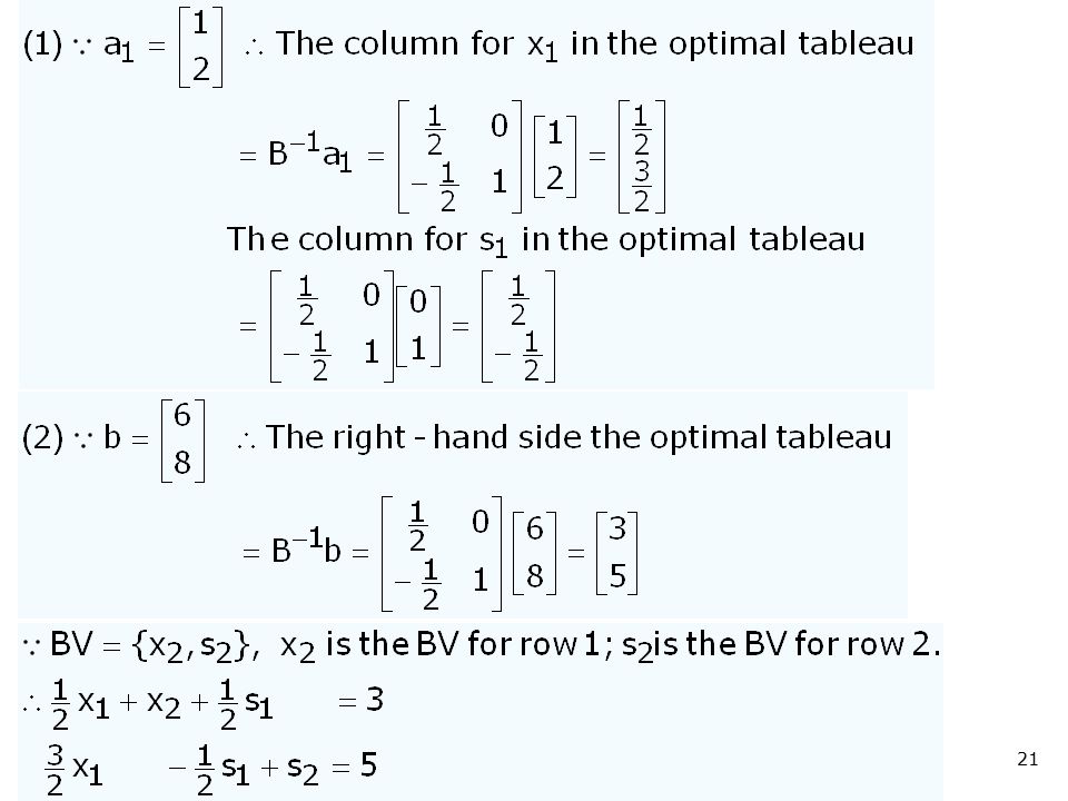
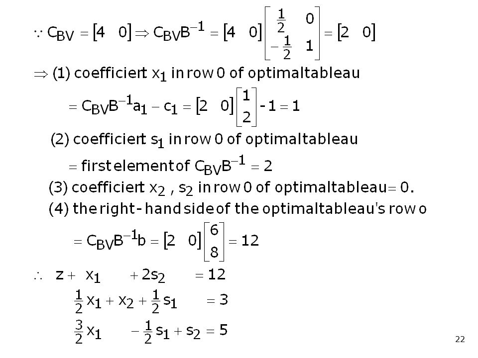
Example 1：compute the optimal tableau
max. z=x1+4x2 s.t. x1+2x2 ≤6 2x1+x2 ≤8 x1,x2 ≥0 The optimal basis is BV={x2,s2} max. z=x1+4x2 s.t. x1+2x2+s =6 2x1+x s2=8 x1,x2, s1, s2 ≥0

Six types of changes in an LP’s parameters change the optimal solution
1.Changing the objective function coefficient of a NBV. 2.Changing the objective function coefficient of a BV. 3.Changing the right-hand side of a constraint. 4.Changing the column of a NBV. 5.Adding a new variable or activity. 6.Adding a new constraint. (Dual Simplex )

Example：Dakota problem (p.140)
max z = 60x1 + 30x2 + 20x3 s.t. 8x1+ 6x x3 + s1 = 48 4x1+ 2x x3 + s2 = 20 2x1+1.5x x3 + s3 = 8 x1, x2, x3 , s1 , s2 , s3 ≥ 0 z +5x1 + 10s2 + 10s3= 280 -2x2 + s1+2s2 - 8s3 = 24 -2x2 + x3 +2s2 - 4s3 = 8 x x s s3= 2 x1, x2, x3 , s1 , s2 , s3 ≥ 0

z = 60x1 + 30x2 + 20x3 +0 s1 + 0s2 +0 s3 8x1+ 6x x3 + s1 = 48 4x1+ 2x x3 + s2 = 20 2x1+1.5x x3 + s3 = 8 x1, x2, x3 , s1 , s2 , s3 ≥ 0 Optimal Basis BV={s1 , x3 , x1}   

    BV Z X RHS 1 CBvB-1A-C CBvB-1b B-1A B-1b
XBv B-1A B-1b     z +5x2 + 10s2 + 10s3= 280 -2x2 + s1+2s2 - 8s3 = 24 -2x2 + x3 +2s2 - 4s3 = 8 x x s s3= 2 x1, x2, x3 , s1 , s2 , s3 ≥ 0

Changing the objective function coefficient of NBV 改變目標函數中“非基本變數”之係數
Z X RHS 1 CBvB-1A-C CBvB-1b XBv B-1A B-1b 若C 改變, 則改變 Ex. c2=25  The current basis is still optimal.

  Ex. c2=40 The current basis is no longer optimal.
Ex. For what value of c2 does the current basis remain optimal ?  Ex. c2=40  The current basis is no longer optimal.

Table 2 (p.278) “Final” (Suboptimal) Dakota Tableau ($40/Table) BV
Ratio z -5x2 +10s2 +10s3 = 280 Z= 280 -2x2 +s1 + 2s2 - 8s3 = 24 s1= 24 None +x3 - 4s3 = 8 x3= 8 x1 +1.25x2 -0.5s2 +1.5s3 = 2 x1 = 2 1.6*

Table 3 (p.278) Optimal Dakota Tableau ($40/Table) BV z + 4x1 + 8s2
= 288 Z= 288 1.6x1 +s1 +1.2s2 -5.6s3 = 27.2 s1= 27.2 +x3 -1.6s3 = 11.2 x3= 11.2 0.8x1 +x2 -0.4s2 +1.2s3 = 1.6 x2 = 1.6

2. Changing the objective function coefficient of a BV 改變目標函數中“基本變數”之係數
若CBv 改變, 則 改變 BV Z X RHS 1 CBvB-1A-C CBvB-1b XBv B-1A B-1b Ex. c1=70, CBv=[ ]  

Ex. For what value of c1 does the current basis remain optimal ?


Ex. c1=100 > 80  The current basis is no longer optimal.

Table 4 (p.281) “Final” (Suboptimal) Tableau if c1=100 BV Ratio z
+55x2 -10s2 +70s3 = 360 Z= 360 - 2x2 +s1 +2s2 - 8s3 = 24 s1= 24 12 +x3 - 4s3 = 8 x3 = 8 4* x1 +1.25x2 -0.5s2 +1.5s3 = 2 x1 = 2 None

Table 5 (p.281) Optimal Dakota Tableau if c1=100 BV z + 45x2 + 5x3
+50s3 = 400 Z= 400 - x3 + s1 - 4s3 = 16 s1= 16 - x2 +0.5x3 + s2 - 2s3 = 4 s2 = 4 x1 + 0.75x2 +0.25x3 +0.5s3 x1 = 4

3. Changing the right-hand side of a constraint 改變限制式的右邊值
BV Z X RHS 1 CBvB-1A-C CBvB-1b XBv B-1A B-1b 若b改變, 則 改變 Ex. b2=22,  The current basis BV is not changed. 

  Ex. For what value of b2 does the current basis BV
remain optimal ?  Ex. b2=30 > 24 The current basis is no longer optimal.  If the RHS of any constraint is negative, then the current basis is infeasible, a new solution must be found.

Table 6 (p.285) “Final” (infeasible) Dakota Tableau if b2 = 30 BV z
+ 5x2 +10s2 +10s3 = 380 Z= 380 - 2x2 +s1 + 2s2 - 8s3 = 24 s1 = 24 +x3 - 4s3 = 8 x3 = 8 x1 +1.25x2 -0.5s2 +1.5s3 = -3 x1 = - 3

4.Changing the column of a NBV 改變非基本變數之行係數(ci and ai均改變)
p.285 4.Changing the column of a NBV 改變非基本變數之行係數(ci and ai均改變) 若A 改變, 則 改變 BV z X RHS 1 CBvB-1A-C CBvB-1b XBv B-1A B-1b Ex.  The current basis is still optimal.

Ex. c2=43,  The current basis is no longer optimal.

Table 7 (p.286) “Final” (Suboptimal) Dakota Tableau for New Method of Making Tables BV Ratio z - 3x2 +10s2 +10s3 = 280 Z= 280 - 7x2 +s1 + 2s2 - 8s3 = 24 s1= 24 None - 4x2 +x3 - 4s3 = 8 x3= 8 x1 + 2x2 -0.5s2 +1.5s3 = 2 x1 = 2 1*

Table 8 (p.278) Optimal Dakota Tableau for New Method of Making Tables
BV z +1.5x1 +9.25s2 +12.25s3 = 283 Z= 283 3.5x1 +s1 +0.25s2 -2.75s3 = 31 s1= 31 2x1 +x3 + s2 - s3 = 12 x3= 12 0.5x1 +x2 -0.25s2 +0.75s3 = 1 x2 = 1

5. Adding a new variable or activity 增加新的活動
BV Z X RHS 1 CBvB-1A-C CBvB-1b XBv B-1A B-1b If current basis will remain optimal if  ≥0 or become nonoptimal if  ≤ 0

Ex. c4=15,  The current basis is still optimal

Exercise: p.288 Dakota problem
1. Show that the current basis remains optimal if c3 satisfies 15≤c3≤22.5. If c3=21, find the new optimal solution. Also, if c3=25, find the new optimal solution. 2. If c1=55, show that the new optimal solution does not produce any desks. 3. Show that if b1≥24, the current basis remains optimal. If b1=30, find the new optimal solution. 4.Show that if tables sell for $50 and use 1 board ft of lumber, 3 finishing hours, and 1.5 carpentry hours, the current basis will no longer be optimal. Find the new optimal solution. 5. Dakota is considering manufacturing home computer tables. It sells for $36 and uses 6 board ft of lumber , 2 finishing hours, and 2 carpentry hours. Should the company manufacture any home computer tables?

Type 1 BV={s1, x3 , x1} Change c3 to 20 + Δ cBVB‑1 = [0 20+Δ 60] = [ Δ 10-4Δ] Coefficient of x2 in row 0 =cBVB‑1a2‑c2 = [0 10+2Δ 10-4Δ ] = 5-2Δ New row 0 is z + (5‑2Δ)x2+(10+2Δ)s2+(10‑4Δ)s3 Current basis remains optimal if (1) 5‑2Δ  0 iff Δ  2.5 (2) Δ 0 iff Δ ‑5 ‑5Δ 2.5 or20‑5  c3  (3)10‑4Δ 0 iff Δ 2.5

Thus current basis remains optimal if ‑5 Δ 2. 5 or 20‑5  c3  20+2
If c3=21 the current solution is still optimal , z increases by 8 to z=288. If c3=25,Δ=5, the tableau for the current optimal basis becomes z ‑5x2 + 20s2 ‑ 10s3 = 320 ‑2x2 + s1 + 2s2 ‑ 8s3 = 24 ‑2x2 + x3 + 2s2 ‑ 4s3 = 8 x x2 ‑ .5s s3 = 2 Eventually we obtain the new optimal solution z= 1000/3, x3= 40/3, x1=x2=0.

p.289 The 100% Rule for Changing objective function coefficient : The 100% Rule Case 1 – All variables whose objective function coefficients are changed have nonzero reduced costs in the optimal row 0. The current basis remains optimal if and only if the objective function coefficient for each variable remains within the allowable range . If the current basis remains optimal, both the values of the decision variables and objective function remain unchanged. If the objective coefficient for any variable is outside the allowable range, the current basis is no longer optimal. Case 2 – At least one variable whose objective function coefficient is changed has a reduced cost of zero.

The 100% Rule for Changing Right-Hand Sides
p.292 The 100% Rule for Changing Right-Hand Sides Case 1 – All constraints whose right-hand sides are being modified are nonbinding constraints. The current basis remains optimal if and only if each rhs remains within its allowable range. Then the values of the decision variables and optimal objective function remain unchanged. If the rhs for any constraint is outside its allowable range, the current basis is no longer optimal. Case 2 – At least one of the constraints whose rhs is being modified is a binding constraint (that is, has zero slack or excess).

6.5 Finding the Dual of an LP
Associated with any LP is another LP called the dual. Knowledge of the dual provides interesting economic and sensitivity analysis insights. When taking the dual of any LP, the given LP is referred to as the primal. If the primal is a max problem, the dual will be a min problem and visa versa. To find the dual to a max problem in which all the variables are required to be nonnegative and all the constraints are ≤ constraints (called normal max problem) the problem may be written as

Finding the Dual of a Normal Max or Min Problem
Table 14 (p.296) Primal LP Dual LP Max n 個變數 m 個限制式 Min 第 i 個限制式第 i 個變數第 j 個變數第 j 個限制式 (相反) (一致)

The dual of a normal max problem is called a normal min problem.
max z = c1x1+ c2x2 +…+ cnxn s.t. a11x1 + a12x2 + … + a1nxn ≤ b1 a21x1 + a22x2 + … + a2nxn ≤ b2 … … … … am1x1 + am2x2 + … + amnxn ≤ bm xj ≥ 0 (j = 1, 2, …,n) The dual of a normal max problem is called a normal min problem. min w = b1y1+ b2y2 +…+ bmym s.t. a11y1 + a21y2 + … + am1ym ≥ c1 a12y1 + a22y2 + … + am2ym ≥ c2 … … … … a1ny1 + a2ny2 + …+ amnym ≥ cn yi ≥ 0 (i = 1, 2, …,m)

主要問題與對偶問題之關係 Max Min 1 限制式 ≤ ≥ 0 變數 2 ≥ ≤ 0 3 = urs 4 5 6

Finding the Dual of a Normal Max or Min Problem
Table 14 (p.296) Example：Dakota problem (Table 15) Example：Diet problem (Table 16) Exercise：problem 1 (p.301)

Table 14 (p.296) max z0 min w x1 x2 … xn y1 a11 a12 a1n ≦ b1 y2 a21
(ym≧ 0) ym am1 am2 anm ≦ bm ≧c1 ≧c2 ≧cn

Table 15 (p.296) max z min w x1 x2 x3 y1 8 6 1 ≦ 48 y2 4 2 1.5 ≦ 20 y3
0.5 ≦ 8 ≧60 ≧30 ≧20

Table 16 (p.297) max z min w x1 x2 x3 x4 y1 400 3 2 ≦ 50 y2 200 4 ≦ 20
150 1 ≦ 30 (y4≧ 0) y4 500 5 ≦ 80 ≧500 ≧6 ≧10 ≧8

Finding the Dual of a Nonnormal LP
Transforming into normal form Normal max problem：step1 ~ 3 Normal min problem：step1 ~ 3 Finding the dual of a nonnormal max problem step1 ~ 2 (p.299), Example：table17-18 Finding the dual of a nonnormal min problem step1 ~ 2 (p.300), Example：table19-20 Exercise：problem 3, 4 (p.301)

6.6 Economic Interpretation of the Dual Problem
Suppose an entrepreneur wants to purchase all of Dakota’s resources. The entrepreneur must determine the price he or she is willing to pay for a unit of each of Dakota’s resources. To determine these prices define: y1 = price paid for 1 boards ft of lumber y2 = price paid for 1 finishing hour y3 = price paid for 1 carpentry hour The resource prices y1, y2, and y3 should be determined by solving the Dakota dual. Example：Dakota dual

In setting resource prices, the prices must be high enough to induce Dakota to sell.
When the primal is a normal max problem, the dual variables are related to the value of resources available to the decision maker. For this reason, dual variables are often referred to as resource shadow prices.

6.7 The Dual Theorem and Its Consequences
p.304 6.7 The Dual Theorem and Its Consequences The Dual Theorem states that the primal and dual have equal optimal objective function values (if the problems have optimal solutions). Lemma 1： Weak duality implies that if for any feasible solution to the primal and an feasible solution to the dual, the w-value for the feasible dual solution will be at least as large as the z-value for the feasible primal solution. (p.305) Any feasible solution to the dual can be used to develop a bound on the optimal value of the primal objective function.

Lemma 2 ：Let be a feasible solution to the primal and be a feasible solution to the dual. If , then x-bar is optimal for the primal and y-bar is optimal for the dual. Lemma 3 ： If the primal is unbounded, then the dual problem is infeasible. Lemma 4 ： If the dual is unbounded, then the primal is infeasible.

The Dual Theorem*** (p.308)
Suppose BV is an optimal basis for the primal. Then cBVB-1 is an optimal solution to the dual. Also 原題的解(x-bar)與對偶題的解(y-bar)存在對應關係，且二者的最佳值相等。

p.313 6.8 Shadow Prices The shadow price of the ith constraint is the amount by which the optimal z-value is improved (increased in a max problem and decreased in a min problem) is we increase bi by 1 (from bi to bi+1). In short, adding points to the feasible region of a max problem cannot decrease the optimal z-value.

6.9 Duality and Sensitivity Analysis
p.323 6.9 Duality and Sensitivity Analysis Assuming that a set of basic variables BV is feasible, then BV is optimal if and only if the associated dual solution (cBVB-1) is dual feasible. This result can be used for an alternative way of doing the following types of sensitivity analysis(6.3, p.276). Change 1：Changing the objective function coefficient of a nonbasic variable. Change 4：Changing the column of a nonbasic variable Change 5：Adding a new activity.

6.10 Complementary Slackness
Theorem 2：Let be a feasible primal solution and be a feasible dual solution. Then x is primal optimal and y is dual optimal if and only if siyi = 0 (i=1, 2, …, m) ejyj = 0 (j=1, 2, …, n)

6.11 The Dual Simplex Method
The dual simplex method (對偶單體法) maintains a non-negative row 0 (dual feasibility) and eventually obtains a tableau in which each right-hand side is non-negative (primal feasibility).

The dual simplex method for a max problem
Step 1:Is the right-hand side of each constraint non negative? If not, go to step 2. Step 2:Choose the most negative basic variable as the variable to leave the basis. The row it is in will be the pivot row. To select the variable that enters the basis, computer the following ratio for each variable xj that has a negative coefficient in the pivot row: Choose the variable with the smallest ratio as the entering variable. Now use EROs to make the entering variable a basic variable in the pivot row. Step 3: If there is any constraint in which the right-hand side is negative and each variable has a non-negative coefficient, then the LP has no feasible solution. If no constraint infeasibility is found, return to step 1.

Three uses of the dual simplex
Finding the new optimal solution after a constraint is added to an LP. (p.330) Finding the new optimal solution after changing a right-hand side of an LP. (p.332) Solving a normal min problem. (p.333)

When a constraint is added one of the following three cases will occur
When a constraint is added one of the following three cases will occur.(p.330) The current optimal solution satisfies the new constraint. The current optimal solution does not satisfy the new constraint, but the LP still has a feasible solution. The additional constraint causes the LP to have no feasible solutions. Case 1 ：x1+x2+x3 ≦ 11 (p.330) Case 2 ：x2 ≧ 1 (p.330, table 33-34) Case 3 ：x1+x2 ≧ 12 (p.331, table 35-38)

A Constraint Is Added to an LP
max z = 60x1 + 30x2 + 20x3 s.t. 8x1+ 6x x3 ≤ 48 4x1+ 2x x3 ≤ 20 2x1+1.5x x3 ≤ 8 x1, x2, x3 ≥ 0 BV z x1 X2 x3 s1 s2 s3 RHS 1 5 10 280 -2 2 -8 24 -4 8 1.25 -0.5 1.5

Case 1 加入限制式 x1+x2+x3 ≤ 11 x1+x2+x3 ≤ 11 ⇒ x1+x2+x3 +s4= 11 1 5 10 280
BV z x1 x2 x3 s1 s2 s3 RHS 1 5 10 280 -2 2 -8 24 -4 8 1.25 -0.5 1.5 x1+x2+x3 ≤ 11 ⇒ x1+x2+x3 +s4= 11 BV z x1 x2 x3 s1 s2 s3 s4 RHS 1 5 10 280 -2 2 -8 24 -4 8 1.25 -0.5 1.5 11

BV z x1 x2 x3 s1 s2 s3 s4 RHS 1 5 10 280 -2 2 -8 24 -4 8 1.25 -0.5 1.5 11 ERO BV z x1 x2 x3 s1 s2 s3 s4 RHS 1 5 10 280 -2 2 -8 24 -4 8 1.25 -0.5 1.5 0.25 0.5 -1.5 9 The current optimal solution remains optimal after the constraint x1+x2+x3 ≤ 11 is added.

Case 2 加入限制式 x2 ≥ 1 x2 ≥ 1 ⇒ -x2 +e4=- 1 1 5 10 280 -2 2 -8 24 -4 8
BV z x1 x2 x3 s1 s2 s3 RHS 1 5 10 280 -2 2 -8 24 -4 8 1.25 -0.5 1.5 x2 ≥ 1 ⇒ -x2 +e4=- 1 TABLE 33 BV z x1 x2 x3 s1 s2 s3 e4 RHS 1 5 10 280 -2 2 -8 24 -4 8 1.25 -0.5 1.5 -1

TABLE 33 EV BV z x1 x2 x3 s1 s2 s3 e4 RHS r 1 5 10 280 -2 2 -8 24 -4 8 1.25 -0.5 1.5 -1 LV ERO TABLE 34 BV z x1 x2 x3 s1 s2 s3 e4 RHS 1 10 5 275 2 -8 -2 26 -4 -1/2 3/4 5/4 -1

Case 3 加入限制式 x1 +x2 ≥ 12 x1 +x2 ≥ 12 ⇒ -x1 -x2 +e4 = - 12 1 5 10 280
BV z x1 x2 x3 s1 s2 s3 RHS 1 5 10 280 -2 2 -8 24 -4 8 1.25 -0.5 1.5 x1 +x2 ≥ 12 ⇒ -x1 -x2 +e4 = - 12 TABLE 35 BV z x1 x2 x3 s1 s2 s3 e4 RHS 1 5 10 280 -2 2 -8 24 -4 8 1.25 -0.5 1.5 -1 -12

TABLE 35 EV BV z x1 x2 x3 s1 s2 s3 e4 RHS 1 5 10 280 -2 2 -8 24 -4 8 1.25 -0.5 1.5 -1 -12 LV TABLE 36 EV BV z x1 x2 x3 s1 s2 s3 e4 RHS 1 5 10 280 -2 2 -8 24 -4 8 1.25 -0.5 1.5 0.25 -10 LV

TABLE 36 EV BV z x1 x2 x3 s1 s2 s3 e4 RHS 1 5 10 280 -2 2 -8 24 -4 8 1.25 -0.5 1.5 0.25 -10 LV TABLE 37 EV BV z x1 x2 x3 s1 s2 s3 e4 RHS 1 10 40 20 80 -1 -2 4 -16 2 -32 LV 12 -0.5 -3

TABLE 37 EV BV z x1 x2 x3 s1 s2 s3 e4 RHS 1 10 40 20 80 -1 -2 4 -16 2 -32 LV 12 -0.5 -3 TABLE 38 BV z x1 x2 x3 s1 s2 s3 e4 RHS 1 10 60 -240 -1 -4 16 -2 32 2 3 -20 -0.5 36

If the right-hand side of a constraint is changed and the current basis becomes infeasible, the dual simplex can be used to find the new optimal solution.(p.332) -Example：finishing hours=30, table 39-40

Changing a RHS of an LP p.332 max z = 60x1 + 30x2 + 20x3
s.t. 8x1+ 6x x3 ≤ 48 4x1+ 2x x3 ≤ 20 2x1+1.5x x3 ≤ 8 x1, x2, x3 ≥ 0 BV z x1 X2 x3 s1 s2 s3 RHS 1 5 10 280 -2 2 -8 24 -4 8 1.25 -0.5 1.5

b2=20→30 TABLE 39 BV z x1 x2 x3 s1 s2 s3 e4 RHS 1 5 10 380 -2 2 -8 44 -4 28 1.25 -0.5 1.5 -3

TABLE 39 EV BV z x1 x2 x3 s1 s2 s3 RHS 1 5 10 380 -2 2 -8 44 -4 28 1.25 -0.5 1.5 -3 LV TABLE 40 BV z x1 x2 x3 s1 s2 s3 RHS 1 20 30 40 320 4 3 -2 32 2 16 -2.5 -3 6

Solving a Normal Min Problem
Min z=x1+2x2 s.t. x1 -2x2 + x3 ≥ 4 2x1 + x2 - x3 ≥ 6 x1 , x2, x3 ≥ 0 Let z’=-z, z’= -x1 - 2x2 z’ + x1 + 2x2 = 0 x1 -2x2 + x3 - e1 = 4 2x1 + x2 - x3 - e2 = 6

Solving a Normal Min Problem
Table 41 z’ + x1 + 2x2 = 0 -x1+2x2 - x3 + e1 = -4 -2x1 - x2 + x3 + e2 = -6 Table 42 BV z x1 x2 x3 e1 e2 RHS 1 2 -1 -4 -2 -6 ratio |1/(-2) | |1/(-1) | min 1.RHS (負值)最小離開, e2 leaving 2.ratio最小進入, x1entering

1.RHS ( 負值)最小離開, e1 leaving 2.ratio最小進入, x3 entering
Table 43 BV z x1 x2 x3 e1 e2 RHS 1 3/2 1/2 -3 5/2 -3/2 -1/2 -1 3 ratio min 1.RHS ( 負值)最小離開, e1 leaving 2.ratio最小進入, x3 entering Table 44 BV z x1 x2 x3 e1 e2 RHS 1 7/3 1/3 -10/3 -5/3 -2/3 2/3 -1/3 - 1/3 10/3 ratio min z’ = -10/3, z = 10/3, x1 = 10/3, x3 = 2/3, x2 = 0

Exercise : p.335 #1 ⇒ Max z=-2x1-x3 s.t. x1 + x2 - x3 ≥ 5
Use the dual simplex method to solve the following LP: Max z=-2x1-x3 s.t. x1 + x x3 ≥ 5 x1 - 2x2 + 4x3 ≥ 8 x1 , x2, x3 ≥ 0 z + 2x1 + x3 = 0 x1 +x2 - x3 - e1 = 5 x1 - 2x2 + 4x3 - e2 = 8 z + 2x1 + x3 = 0 - x1 - x2 + x3 + e1 = ‑5 - x1 + 2x2 - 4x3 + e2 = -8 ⇒

Exercise : p.335 #1 z + 2x1 + x3 = 0 - x1 - x2 + x3 + e1 = ‑5
BV z x1 x2 x3 e1 e2 RHS 1 2 -1 -5 -4 -8 ratio |2/(-1) | |1/(-4) | min 1.RHS ( 負值)最小離開, e2 leaving 2.ratio最小進入, x3entering

1.RHS (負值)最小離開, e1 leaving 2.ratio最小進入, x2 entering BV z x1 x2 x3 e1
-1 -5 -4 -8 ratio |2/(-1) | |1/(-4) | min BV z x1 x2 x3 e1 e2 RHS 1 7/4 1/2 1/4 -2 -5/4 -1/2 -7 -1/4 2 ratio min 1.RHS (負值)最小離開, e1 leaving 2.ratio最小進入, x2 entering

z = ‑9, x2 = 14, x3 = 9 BV z x1 x2 x3 e1 e2 RHS 1 1/2 -9 5/2 -2 -1/2
-9 5/2 -2 -1/2 14 3/2 -1 9 z = ‑9, x2 = 14, x3 = 9

主要單體法與對偶單體法知差異 (Max problem)
差異項目主要單體法對偶單體法 1 0列不受正負限制* 均為非負值 2 RHS 3 判斷最佳解 0列均為非負值 RHS均為非負值 4 選擇進入變數最負0列最負RHS 5 Ratio Min{RHS/正係數} Min{|0列係數/負係數|} *最佳解除外

對偶問題 Max. Z=x1 - 2x2 + 3x3 s.t. 2x1 + x2 + 4x3 - x4 ≦ - 4
x1≧0, x2≧0, x3 urs, x4≦0 --- y1 --- y2 --- y3 Min. w= -4y1 +5y2 + 6y3 s.t. 2y1 - y2 + y3 ≦ 1 y1 + 2y2 - 3y3 ≧ -2 4y y2 + 2y3 = 3 -y1 + 4y2 + y3 ≦ 0 y1≧0, y2 ≦ 0, y3 urs

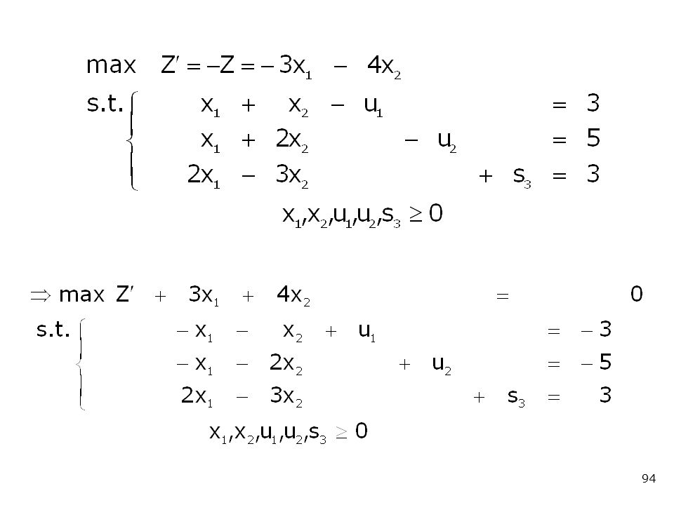
求線性規劃之對偶問題

故x1=1,x2=2,u1=0,u2=0,s3=7 Z 有最大值 11，即 Z 有最小值11

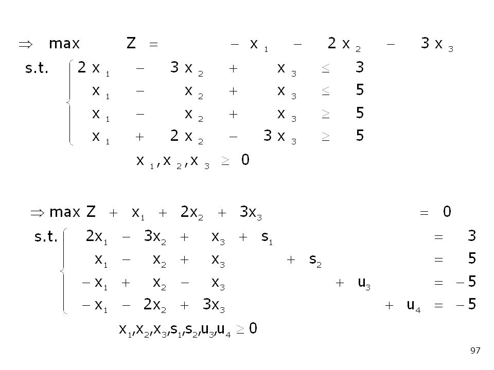
利用對偶單體法求解下LP問題

故 x1 = 6, x2 = 4, x3 = 3, s1 = s2 = u3 = u4 =0 時， Z 有最大值 23

Chapter 6 Sensitivity Analysis & Duality (敏感度分析 & 對偶)

Similar presentations

Presentation on theme: "Chapter 6 Sensitivity Analysis & Duality (敏感度分析 & 對偶)"— Presentation transcript:

Similar presentations

About project

Feedback

Log in

Auth with social network:

Chapter 6 Sensitivity Analysis & Duality (敏感度分析 & 對偶)

Similar presentations

Presentation on theme: "Chapter 6 Sensitivity Analysis & Duality (敏感度分析 & 對偶)"— Presentation transcript:

Similar presentations

About project

Feedback