Download presentation
Presentation is loading. Please wait.

2
Chapter 4 Forecasting

3
Production Planning

4
Overview What is forecasting? Types of forecasts 7 steps of forecasting Qualitative forecasting

5
Overview Quantitative forecasting Time-series forecasting Naïve Moving average Exponential smoothing Seasonal variations Associative methods Monitoring and Controlling Forecasts

6
What is forecasting? Sales will be $200 Million! Could be a prediction based on historical data and mathematical models Could be a prediction based on expertise and intuition Forecasting - Is the art and science of predicting the future Could be a prediction based on both a model and a manager’s expertise

7
7 Steps to a Forecast Determine the use of the forecast Select the items to be forecast Determine the time horizon of the forecast Select the forecasting model(s) Gather the data Make the forecast Validate and implement results
 Gather the data Make the forecast Validate and implement results")
8
Realities of Forecasting Forecasts never perfect and seldom correct. Most forecasting methods assume that there is some underlying stability in the system Both product family and aggregated product forecasts are more accurate than individual product forecasts

9
Demand Forecasts OM manager is primarily interested in demand forecasts (as opposed to economic forecasts and technological forecasts) Underlying basis of all business decisions Production Inventory Personnel Facilities
 Underlying basis of all business decisions Production Inventory Personnel Facilities")
10
Demand Forecast Applications Time Horizon Medium TermLong Term Short Term (3 months–(more than Application(0–3 months) 3 years) 3 years) Forecast quantity Decision area Forecasting technique
 3 years) 3 years) Forecast quantity Decision area Forecasting technique")
11
Demand Forecast Applications Time Horizon Medium TermLong Term Short Term (3 months–(more than Application(0–3 months) 2 years) 2 years) Forecast quantityIndividual products or services Decision areaInventory management Final assembly scheduling Workforce scheduling Master production scheduling ForecastingTime series techniqueAssociative
 2 years) 2 years) Forecast quantityIndividual products or services Decision areaInventory management Final assembly scheduling Workforce scheduling Master production scheduling ForecastingTime series techniqueAssociative")
12
Demand Forecast Applications Time Horizon Medium TermLong Term Short Term (3 months–(more than Application(0–3 months) 2 years) 2 years) Forecast quantityIndividualTotal sales products orGroups or families servicesof products or services Decision areaInventoryStaff planning managementProduction Final assemblyplanning schedulingMaster production Workforcescheduling schedulingPurchasing Master productionDistribution scheduling ForecastingTime seriesAssociative techniqueAssociative
 2 years) 2 years) Forecast quantityIndividualTotal sales products orGroups or families servicesof products or services Decision areaInventoryStaff planning managementProduction Final assemblyplanning schedulingMaster production Workforcescheduling schedulingPurchasing Master productionDistribution scheduling ForecastingTime seriesAssociative techniqueAssociative")
13
Demand Forecast Applications Time Horizon Medium TermLong Term Short Term (3 months–(more than Application(0–3 months) 2 years) 2 years) Forecast quantityIndividualTotal salesTotal sales products orGroups or families servicesof products or services Decision areaInventoryStaff planningFacility location managementProductionCapacity Final assemblyplanningplanning schedulingMaster productionProcess Workforceschedulingmanagement schedulingPurchasing Master productionDistribution scheduling ForecastingTime seriesAssociativeAssociative techniqueAssociative
 2 years) 2 years) Forecast quantityIndividualTotal salesTotal sales products orGroups or families servicesof products or services Decision areaInventoryStaff planningFacility location managementProductionCapacity Final assemblyplanningplanning schedulingMaster productionProcess Workforceschedulingmanagement schedulingPurchasing Master productionDistribution scheduling ForecastingTime seriesAssociativeAssociative techniqueAssociative")
14
Overview of Qualitative Methods READ in TEXT (p. 81-82) Jury of executive opinion Pool opinions of high-level executives, sometimes augment by statistical models Sales force composite Estimates from individual salespersons are reviewed for reasonableness, then aggregated Delphi method Panel of experts, queried iteratively Consumer Market Survey Ask the customer
 Jury of executive opinion Pool opinions of high-level executives, sometimes augment by statistical models Sales force composite Estimates from individual salespersons are reviewed for reasonableness, then aggregated Delphi method Panel of experts, queried iteratively Consumer Market Survey Ask the customer.")
15
Patterns of Demand

16
Quantity Time

17
Patterns of Demand Quantity Time (a) Random: Data cluster about a horizontal line.
 Random: Data cluster about a horizontal line.")
18
Patterns of Demand Quantity Time (b) Trend: Data consistently increase or decrease over a period of time.
 Trend: Data consistently increase or decrease over a period of time.")
19
Patterns of Demand Quantity |||||||||||| JFMAMJJASOND Months (c) Seasonal: Data consistently show peaks and valleys at the same time each year. Year 1

20
Patterns of Demand Quantity |||||||||||| JFMAMJJASOND Months Year 1 Year 2 (c) Seasonal: Data consistently show peaks and valleys at the same time each year.
 Seasonal: Data consistently show peaks and valleys at the same time each year.")
21
Patterns of Demand Quantity |||||| 123456 Years (c) Cyclical: Data reveal gradual increases and decreases over extended periods.
 Cyclical: Data reveal gradual increases and decreases over extended periods.")
22
Overview of Quantitative Methods Naïve approach Moving averages Exponential smoothing Linear regression Time-series Models – no trend, seasonal, or cyclical fluctuations Associative models

23
Set of evenly spaced numerical data Obtained by observing response variable at regular time periods Forecast based only on past values Assumes that factors influencing past and present will continue influence in future Example Year:19931994199519961997 Sales:78.763.589.793.292.1 What is a Time Series?

24
Naïve Approach Assumes demand in next period is the same as demand in most recent period e.g., If May sales were 48, then June sales will be 48 Sometimes cost effective & efficient

25
Moving Average Approach MA is a series of arithmetic means Used if little or no trend Used often for smoothing Provides overall impression of data over time MA n n Demand in Previous Periods Periods

26
Time-Series Methods Simple Moving Averages Patient arrivals have been recorded at a medical clinic over the past 28 weeks. Want to predict the number of patient arrivals for the 29 th week.

27
Time-Series Methods Simple Moving Averages Week 450 — 430 — 410 — 390 — 370 — Patient arrivals |||||| 051015202530 Patient arrivals

28
Time-Series Methods Simple Moving Averages Week 450 — 430 — 410 — 390 — 370 — |||||| 051015202530 Actual patient arrivals Patient arrivals

29
Time-Series Methods Simple Moving Averages Week 450 — 430 — 410 — 390 — 370 — |||||| 051015202530 Actual patient arrivals Patient arrivals -No trend -No seasonal variation -No cycle

30
Time-Series Methods Simple Moving Averages Actual patient arrivals 450 — 430 — 410 — 390 — 370 — Week |||||| 051015202530 Patient arrivals

31
Time-Series Methods Simple Moving Averages Actual patient arrivals Actual patient arrivals 450 — 430 — 410 — 390 — 370 — Week |||||| 051015202530 Patient WeekArrivals 1400 2380 3411 Patient arrivals

32
Time-Series Methods Simple Moving Averages Actual patient arrivals Actual patient arrivals 450 — 430 — 410 — 390 — 370 — Week |||||| 051015202530 Patient WeekArrivals 1400 2380 3411 Patient arrivals

33
Time-Series Methods Simple Moving Averages Actual patient arrivals Week 450 — 430 — 410 — 390 — 370 — |||||| 051015202530 Patient WeekArrivals 1400 2380 3411 F 4 = 411 + 380 + 400 3 Patient arrivals F 4 = 397.0

34
Time-Series Methods Simple Moving Averages Actual patient arrivals 450 — 430 — 410 — 390 — 370 — Week |||||| 051015202530 Patient WeekArrivals 1400 2380 3411 F 4 = 397.0 Patient arrivals

35
Time-Series Methods Simple Moving Averages Actual patient arrivals Week 450 — 430 — 410 — 390 — 370 — |||||| 051015202530 Patient WeekArrivals 2380 3411 4415 F 5 = 415 + 411 + 380 3 Patient arrivals

36
Time-Series Methods Simple Moving Averages Actual patient arrivals 450 — 430 — 410 — 390 — 370 — Week |||||| 051015202530 Patient WeekArrivals 2380 3411 4415 F 5 = 402.0 Patient arrivals

37
Time-Series Methods Simple Moving Averages 450 — 430 — 410 — 390 — 370 — Week |||||| 051015202530 Actual patient arrivals Patient arrivals Go To Excel

38
Time-Series Methods Simple Moving Averages 450 — 430 — 410 — 390 — 370 — Week |||||| 051015202530 Actual patient arrivals 3-week MA forecast Patient arrivals

39
Time-Series Methods Simple Moving Averages Week 450 — 430 — 410 — 390 — 370 — |||||| 051015202530 Actual patient arrivals 3-week MA forecast 6-week MA forecast Patient arrivals

40
WEIGHTED Moving Averages SKIP

41
Increasing n makes forecast less sensitive to changes Do not forecast trend well Require much historical data © 1984-1994 T/Maker Co. Disadvantages of Moving Average Methods

42
Form of weighted moving average Weights decline exponentially Most recent data weighted most Requires smoothing constant ( ) Ranges from 0 to 1 Subjectively chosen Involves little record keeping of past data Exponential Smoothing Method
 Ranges from 0 to 1 Subjectively chosen Involves little record keeping of past data Exponential Smoothing Method")
43
Time-Series Methods Exponential Smoothing 450 — 430 — 410 — 390 — 370 — Week |||||| 051015202530 Exponential Smoothing = 0.10 F t +1 = F t + (D t – F t ) Patient arrivals
 Patient arrivals")
44
Time-Series Methods Exponential Smoothing 450 — 430 — 410 — 390 — 370 — Week |||||| 051015202530 Exponential Smoothing = 0.10 F 3 = 390 (Given) D 3 = 411 F t +1 = F t + (D t – F t ) Patient arrivals F 4 = 390 + 0.10(411-390)
 D 3 = 411 F t +1 = F t + (D t – F t ) Patient arrivals F 4 = ( )")
45
Time-Series Methods Exponential Smoothing 450 — 430 — 410 — 390 — 370 — Week |||||| 051015202530 F 4 = 392.1 Exponential Smoothing = 0.10 F 3 = 390 (Given) D 3 = 411 F t +1 = F t + (D t – F t ) Patient arrivals
 D 3 = 411 F t +1 = F t + (D t – F t ) Patient arrivals")
46
Time-Series Methods Exponential Smoothing Week 450 — 430 — 410 — 390 — 370 — |||||| 051015202530 F 4 = 392.1 D 4 = 415 Exponential Smoothing = 0.10 F 4 = 392.1 F 5 = 394.4 F t +1 = F t + (D t – F t ) Patient arrivals
 Patient arrivals")
47
Time-Series Methods Exponential Smoothing Week 450 — 430 — 410 — 390 — 370 — |||||| 051015202530 Patient arrivals

48
Time-Series Methods Exponential Smoothing 450 — 430 — 410 — 390 — 370 — Patient arrivals Week |||||| 051015202530 Exponential smoothing = 0.10 Go To Excel

49
Time-Series Methods Exponential Smoothing 450 — 430 — 410 — 390 — 370 — Patient arrivals Week |||||| 051015202530 3-week MA forecast Exponential smoothing = 0.10

50
Exponential smoothing with trend adjustment SKIP Trend projection (p. 93-96) Regression analysis
 Regression analysis.")
51
Time-Series Methods Seasonal Influences

52
QuarterYear 1Year 2Year 3Year 4 14570100100 2335370585725 35205908301160 4100170285215 Total1000120018002200 Average250300450550 Time-Series Methods Seasonal Influences

53
QuarterYear 1Year 2Year 3Year 4 14570100100 2335370585725 35205908301160 4100170285215 Total1000120018002200 Average250300450550 Seasonal Index = Actual Demand Average Demand Time-Series Methods Seasonal Influences Projected Annual Demand = 2600 Average Quarterly Demand = 2600/4 = 650

54
QuarterYear 1Year 2Year 3Year 4 14570100100 2335370585725 35205908301160 4100170285215 Total1000120018002200 Average250300450550 Seasonal Index = Actual Demand Average Demand Time-Series Methods Seasonal Influences

55
QuarterYear 1Year 2Year 3Year 4 14570100100 2335370585725 35205908301160 4100170285215 Total1000120018002200 Average250300450550 Seasonal Index = = 0.18 45 250 Time-Series Methods Seasonal Influences

56
Quarter Year 1 Year 2 Year 3 Year 4 145/250 = 0.1870/300 = 0.23100/450 = 0.22100/550 = 0.18 2335/250 = 1.34370/300 = 1.23585/450 = 1.30725/550 = 1.32 3520/250 = 2.08590/300 = 1.97830/450 = 1.841160/550 = 2.11 4100/250 = 0.40170/300 = 0.57285/450 = 0.63215/550 = 0.39 Time-Series Methods Seasonal Influences

57
Quarter Year 1 Year 2 Year 3 Year 4 145/250 = 0.1870/300 = 0.23100/450 = 0.22100/550 = 0.18 2335/250 = 1.34370/300 = 1.23585/450 = 1.30725/550 = 1.32 3520/250 = 2.08590/300 = 1.97830/450 = 1.841160/550 = 2.11 4100/250 = 0.40170/300 = 0.57285/450 = 0.63215/550 = 0.39 QuarterAverage Seasonal Index 1(0.18 + 0.23 + 0.22 + 0.18)/4 = 0.20 2 3 4 Time-Series Methods Seasonal Influences
/4 = Time-Series Methods Seasonal Influences")
58
Quarter Year 1 Year 2 Year 3 Year 4 145/250 = 0.1870/300 = 0.23100/450 = 0.22100/550 = 0.18 2335/250 = 1.34370/300 = 1.23585/450 = 1.30725/550 = 1.32 3520/250 = 2.08590/300 = 1.97830/450 = 1.841160/550 = 2.11 4100/250 = 0.40170/300 = 0.57285/450 = 0.63215/550 = 0.39 QuarterAverage Seasonal Index 1(0.18 + 0.23 + 0.22 + 0.18)/4 = 0.20 2(1.34 + 1.23 + 1.30 + 1.32)/4 = 1.30 3(2.08 + 1.97 + 1.84 + 2.11)/4 = 2.00 4(0.40 + 0.57 + 0.63 + 0.39)/4 = 0.50 Time-Series Methods Seasonal Influences
/4 = ( )/4 = ( )/4 = ( )/4 = 0.50 Time-Series Methods Seasonal Influences")
59
Quarter Year 1 Year 2 Year 3 Year 4 145/250 = 0.1870/300 = 0.23100/450 = 0.22100/550 = 0.18 2335/250 = 1.34370/300 = 1.23585/450 = 1.30725/550 = 1.32 3520/250 = 2.08590/300 = 1.97830/450 = 1.841160/550 = 2.11 4100/250 = 0.40170/300 = 0.57285/450 = 0.63215/550 = 0.39 QuarterAverage Seasonal IndexForecast 1(0.18 + 0.23 + 0.22 + 0.18)/4 = 0.20 2(1.34 + 1.23 + 1.30 + 1.32)/4 = 1.30 3(2.08 + 1.97 + 1.84 + 2.11)/4 = 2.00 4(0.40 + 0.57 + 0.63 + 0.39)/4 = 0.50 Projected Annual Demand = 2600 Average Quarterly Demand = 2600/4 = 650 Time-Series Methods Seasonal Influences
/4 = ( )/4 = ( )/4 = ( )/4 = 0.50 Projected Annual Demand = 2600 Average Quarterly Demand = 2600/4 = 650 Time-Series Methods Seasonal Influences")
60
Quarter Year 1 Year 2 Year 3 Year 4 145/250 = 0.1870/300 = 0.23100/450 = 0.22100/550 = 0.18 2335/250 = 1.34370/300 = 1.23585/450 = 1.30725/550 = 1.32 3520/250 = 2.08590/300 = 1.97830/450 = 1.841160/550 = 2.11 4100/250 = 0.40170/300 = 0.57285/450 = 0.63215/550 = 0.39 QuarterAverage Seasonal IndexForecast 1(0.18 + 0.23 + 0.22 + 0.18)/4 = 0.20650(0.20) =130 2(1.34 + 1.23 + 1.30 + 1.32)/4 = 1.30 3(2.08 + 1.97 + 1.84 + 2.11)/4 = 2.00 4(0.40 + 0.57 + 0.63 + 0.39)/4 = 0.50 Projected Annual Demand = 2600 Average Quarterly Demand = 2600/4 = 650 Time-Series Methods Seasonal Influences
/4 = (0.20) =130 2( )/4 = ( )/4 = ( )/4 = 0.50 Projected Annual Demand = 2600 Average Quarterly Demand = 2600/4 = 650 Time-Series Methods Seasonal Influences")
61
Quarter Year 1 Year 2 Year 3 Year 4 145/250 = 0.1870/300 = 0.23100/450 = 0.22100/550 = 0.18 2335/250 = 1.34370/300 = 1.23585/450 = 1.30725/550 = 1.32 3520/250 = 2.08590/300 = 1.97830/450 = 1.841160/550 = 2.11 4100/250 = 0.40170/300 = 0.57285/450 = 0.63215/550 = 0.39 QuarterAverage Seasonal IndexForecast 1(0.18 + 0.23 + 0.22 + 0.18)/4 = 0.20650(0.20) =130 2(1.34 + 1.23 + 1.30 + 1.32)/4 = 1.30650(1.30) =845 3(2.08 + 1.97 + 1.84 + 2.11)/4 = 2.00650(2.00) =1300 4(0.40 + 0.57 + 0.63 + 0.39)/4 = 0.50650(0.50) =325 Time-Series Methods Seasonal Influences
/4 = (0.20) =130 2( )/4 = (1.30) =845 3( )/4 = (2.00) =1300 4( )/4 = (0.50) =325 Time-Series Methods Seasonal Influences")
62
Remember Regression Analysis?

63
Dependent variable Independent variable X Y

64
Remember Regression Analysis? Dependent variable Independent variable X Y

65
Remember Regression Analysis? Dependent variable Independent variable X Y Regression equation: Y = a + bX

66
Remember Regression Analysis? Dependent variable Independent variable X Y Actual value of Y Value of X used to estimate Y Regression equation: Y = a + bX

67
Remember Regression Analysis? Dependent variable Independent variable X Y Actual value of Y Estimate of Y from regression equation Value of X used to estimate Y Regression equation: Y = a + bX

68
Remember Regression Analysis? Dependent variable Independent variable X Y Actual value of Y Estimate of Y from regression equation Value of X used to estimate Y Deviation, or error { Regression equation: Y = a + bX

69
Regression analysis in forecasting Two applications of regressions analysis in forecasting Time-series data Independent variable is time Dependent variable is the variable that you want to forecast (i.e. demand) Data is not time-series Independent variable is a known variable that can be used to predict (i.e. advertising dollars, customer population) Dependent variable is the variable that you want to forecast (i.e. demand) Regression analysis is the same in both applications
 Data is not time-series Independent variable is a known variable that can be used to predict (i.e. advertising dollars, customer population) Dependent variable is the variable that you want to forecast (i.e. demand) Regression analysis is the same in both applications.")
70
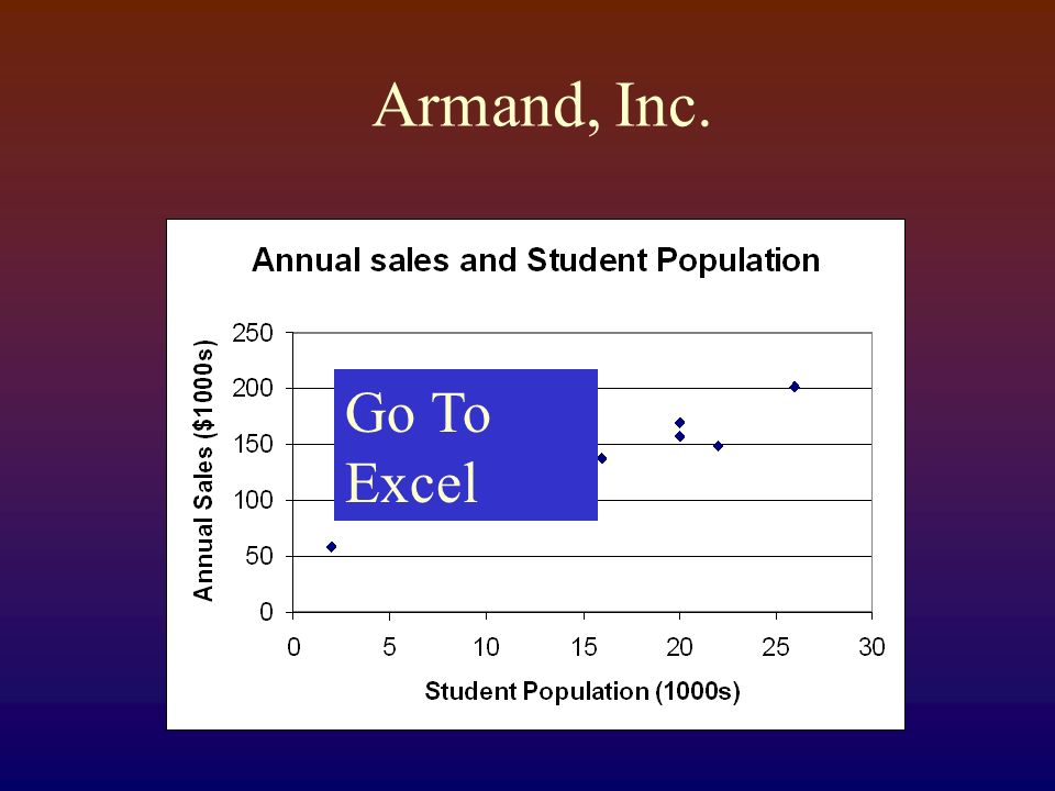
Armand, Inc.: Regression Analysis Armand, Inc. is a chain of Italian restaurants located in a five-state area. The most successful locations have been near college campuses. Prior to opening a new restaurant, management requires a forecast of the yearly sales revenues. Such an estimate is used in planning the restaurant capacity, personnel requirements, and to see if the operations costs are smaller than the predicted revenue.

71
Armand, Inc.

73
Go To Excel

74
Armand, Inc. Intercept Coefficient for Student Population

75
Armand, Inc. Forecast the Annual Sales if the student population is 20,000.

76
Armand, Inc. Forecast the Annual Sales if the student population is 20,000. Forecast is : $160,000

77
Forecasting accuracy “I think there is a world market for about FIVE computers.” —Thomas J. Watson, chairman of IBM, 1943

78
Forecast accuracy IBM 1994 $700 million inventory of OBSOLETE PCs that took 6 months to unload. Reaction: too conservative when releasing the new Aptiva home PCs. New models sold out before the holiday season had begun.

79
Measuring the quality of forecasting MAD – mean absolute deviation MSE – mean square error

80
Your Turn Demand for April-September is given. Determine the exponential smoothing forecasts for those April. Forecast for Mar was 58 Demand for Mar was 60. Determine the regression equation forecasts for those April. X is the number of months in the future (for April, X = 1)
.")
81
Your Turn Demand Exponential Smoothing alpha = 0.2 Regression Y = 54 + 3.9X April60 May55 June75 July60 August80 September75 Calculate for APRIL: Exponential smoothing forecast Regression forecast Forecast for Mar was 58 Demand for Mar was 60. X is the number of months in the future (for April, X = 1)
.")
82
Your Turn Demand Exponential Smoothing alpha = 0.20 Regression Y = 54 + 3.9X April6058.41.657.92.1 May June July August September

83
Your Turn Demand Exponential Smoothing alpha = 0.20 Exp Smooth abs(forecast error) Regression Y = 54 + 3.9X Regression abs(forecast error) April6058.457.9 May5558.761.8 June7558.065.7 July6061.469.6 August8061.173.5 September7564.977.4 MAD = Calculate abs(forecast error) for April
 Regression Y = X Regression abs(forecast error) April May June July August September MAD = Calculate abs(forecast error) for April")
84
Your Turn Demand Exponential Smoothing alpha = 0.20 Regression Y = 54 + 3.9X April6058.41.657.92.1 May5558.761.8 June7558.065.7 July6061.469.6 August8061.173.5 September7564.977.4 MAD =

85
Your Turn Demand Exponential Smoothing alpha = 0.20 Regression Y = 54 + 3.9X April6058.41.657.92.1 May5558.73.761.86.8 June7558.017.065.79.3 July6061.41.469.69.6 August8061.118.973.56.5 September7564.910.177.42.4 MAD = Calculate MAD for each.

86
Your Turn Demand Exponential Smoothing alpha = 0.20 Regression Y = 54 + 3.9X April6058.41.657.92.1 May5558.73.761.86.8 June7558.017.065.79.3 July6061.41.469.69.6 August8061.118.973.56.5 September7564.910.177.42.4 MAD =8.8MAD =6.12

87
Third Wave Research Group - offers marketing software and databases - Forecasts sales for specific -Market areas -Products -segments

88
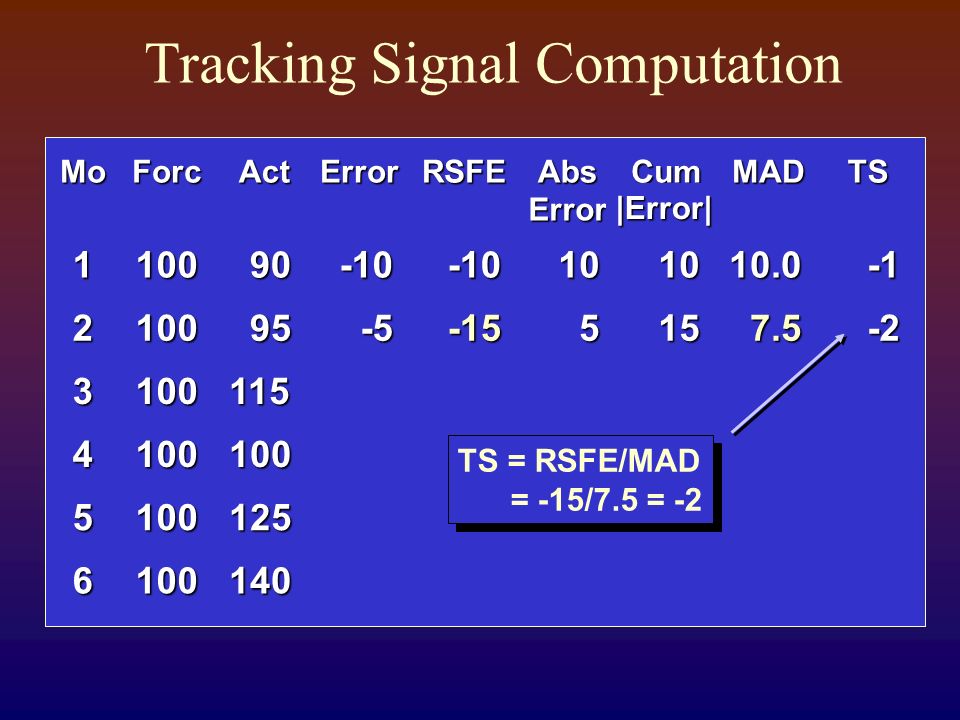
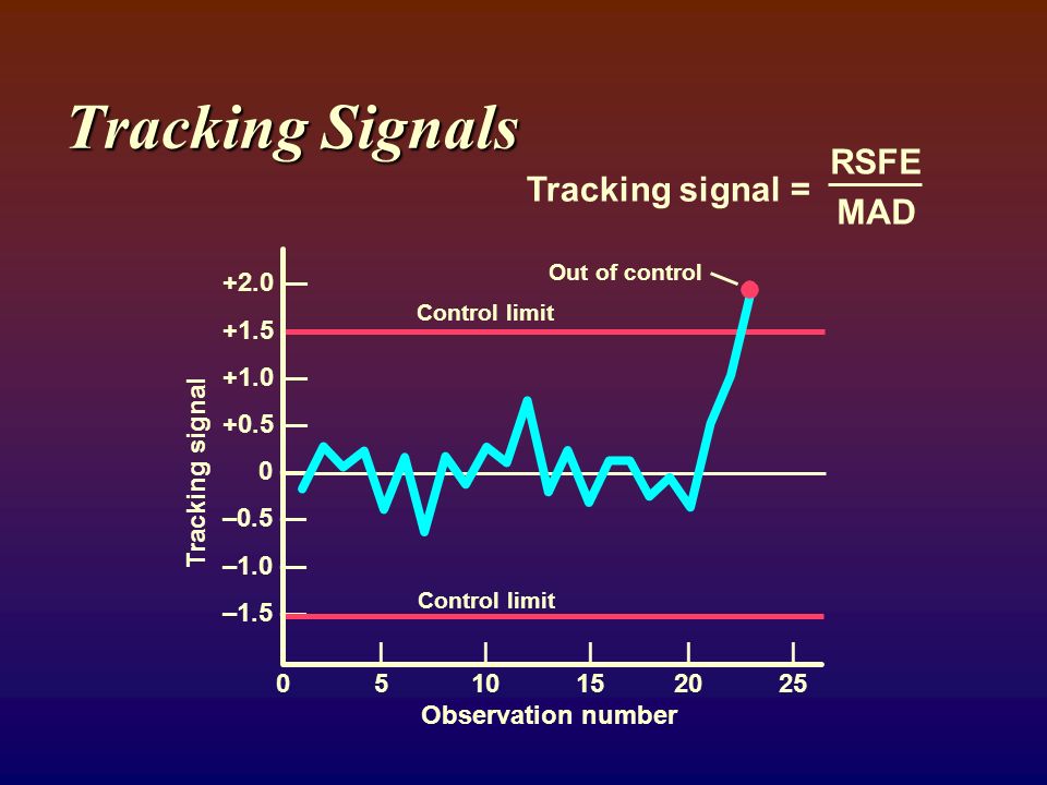
Tracking Signals

89
Tracking signal = RSFE MAD +2.0 — +1.5 — +1.0 — +0.5 — 0 — –0.5 — –1.0 — –1.5 — ||||| 0510152025 Observation number Tracking signal Control limit

90
Tracking Signals Tracking signal = RSFE MAD +2.0 — +1.5 — +1.0 — +0.5 — 0 — –0.5 — –1.0 — –1.5 — ||||| 0510152025 Observation number Tracking signal Control limit Out of control

91
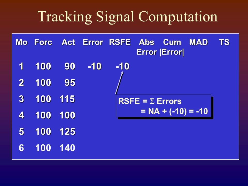
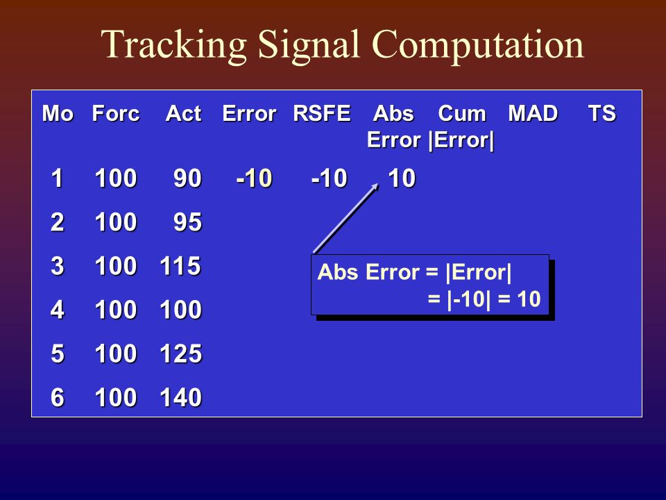
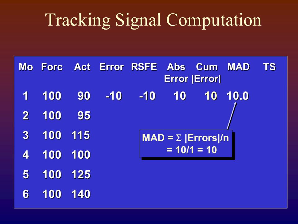
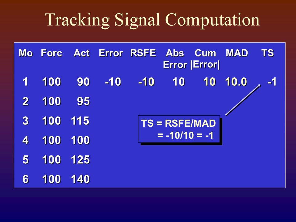
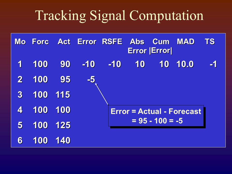
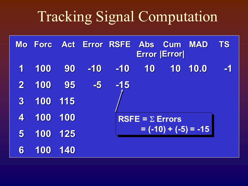
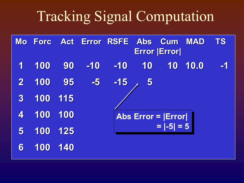
Tracking Signal Computation

104
Tracking Signals Tracking signal = RSFE MAD +2.0 — +1.5 — +1.0 — +0.5 — 0 — –0.5 — –1.0 — –1.5 — ||||| 0510152025 Observation number Tracking signal Control limit Out of control

105
Demand Forecast Applications Time horizons Short term0 – 3 monthsDay to day More accurate Medium term3 months – 3 yearsSales & Production planning Budgeting Long termOver 3 yearsLong term projects Facility planning New products

Similar presentations